This vignette focuses on the Dyadic Score Model (DSM) for distinguishable dyads and its relationship to the distinguishable Actor-Partner Interdependence Model (APIM). The DSM expresses associations in terms of the dyad’s shared level and the directional difference between partners (Iida et al. 2018).
For the broader package workflow and an overview of the available model-specific vignettes, including the Actor-Partner Interdependence Model and Dyad-Individual Model, see the online package overview.
Preparing DSM Data
A DSM requires an explicitly declared direction. This direction
should be substantively meaningful when the directional coefficients are
interpreted. Here, c("female", "male") defines every
difference as female minus male.
Here
and
denote provided support centered with the pooled mean from complete
predictor pairs. prepare_dyad_data() creates the
corresponding DSM dyad-mean column; using the original zero requires
shifting it manually.
cross_dsm_data <- dyadMLM::prepare_dyad_data(
  dyads_cross,
  dyad = coupleID,
  member = personID,
  role = gender,
  predictors = provided_support,
  model_types = "dsm",
  # All three observed compositions in `dyads_cross` are detected and retained by
  # default. This example focuses on `female-male` dyads, so we restrict the
  # analysis here.
  keep_compositions = "female-male",
  dsm_role_order = c("female", "male")
)

print(cross_dsm_data, n = 4)
#> # dyadMLM data
#> # Rows: 240 | Dyads: 120 | Intensive longitudinal: no
#> # Structure: dyad = coupleID, member = personID, role = gender
#> # DSM direction: female - male
#> #
#> # Dyad compositions:
#> # female_x_male distinguishable 120 dyads
#> #
#> # Added columns:
#> #   .composition              inferred dyad composition
#> #   .composition_role         composition-specific member role
#> #   .is_{role}                composition-role indicator columns
#> #   .dsm_role_contrast        DSM role contrast: +0.5 for the first declared
#> #                             role and -0.5 for the second declared role
#> #   .{pred}_dyad_mean_gmc     dyad-mean predictor: dyad's average predictor
#> #                             level, grand-mean centered
#> #   .{pred}_within_dyad_diff  DSM signed predictor difference: first declared
#> #                             role minus second declared role
#> #
#> # A tibble: 240 × 12
#>   personID coupleID gender closeness provided_support .composition
#>      <int>    <int> <fct>      <dbl>            <dbl> <fct>
#> 1        1        1 female      4.71             4.49 female_x_male
#> 2        2        1 male        4.61             4.76 female_x_male
#> 3        3        2 female      6.69             4.09 female_x_male
#> 4        4        2 male        5.98             6.20 female_x_male
#> # ℹ 236 more rows
#> # ℹ 6 more variables: .composition_role <fct>, .is_female <dbl>,
#> #   .is_male <dbl>, .dsm_role_contrast <dbl>,
#> #   .provided_support_dyad_mean_gmc <dbl>,
#> #   .provided_support_within_dyad_diff <dbl>
With this notation, dyadMLM creates the equivalent
coordinates:
.provided_support_dyad_mean_gmc.provided_support_within_dyad_diff.dsm_role_contrastfor female and for male.
The common centering shift cancels from the signed difference. Both predictor scores are repeated on the member rows; the outcome remains unchanged. APIM GMC uses all retained non-missing values, whereas DSM uses complete pairs, so their constants may differ with one-sided missingness.
Cross-Sectional Gaussian DSM
For a cross-sectional Gaussian DSM, a correlated dyad random intercept and role-contrast slope represent unexplained outcome-level and outcome-difference variance.
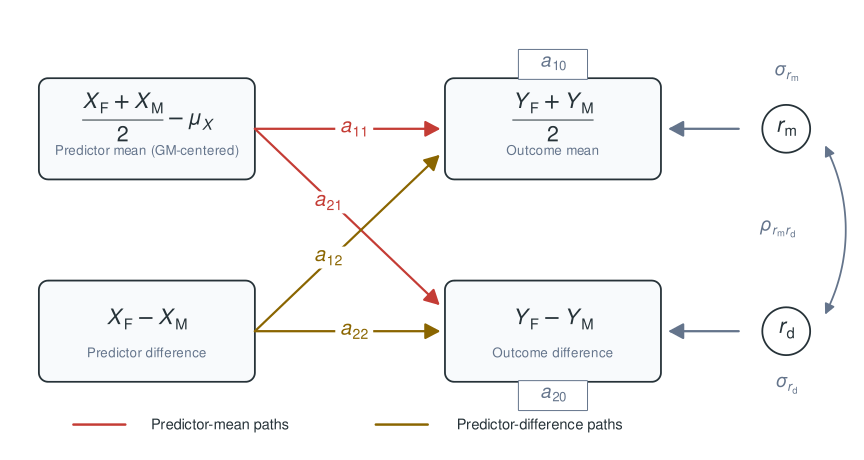
Conceptual cross-sectional DSM. Predictor mean and predictor difference each predict both outcome scores.
The same model can be displayed in the individual-member rows used by the long-format multilevel model.
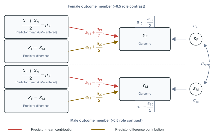
Individual-level representation of the cross-sectional DSM used for the long-format multilevel model. The centered predictor mean and female-minus-male predictor difference appear on both member rows. For the female outcome, the intercept and slopes add one-half of the corresponding outcome-difference parameters. For the male outcome, they subtract one-half. The female and male residuals may have different variances and covary.
The path labels correspond directly to the terms in the model below:
dsm_model <- glmmTMB::glmmTMB(
  closeness ~

    # Outcome-level intercept
    1 +

    # Predictor level -> outcome level (a11)
    .provided_support_dyad_mean_gmc +

    # Predictor difference -> outcome level (a12)
    .provided_support_within_dyad_diff +

    # Outcome-difference intercept (a20)
    .dsm_role_contrast +

    # Predictor level -> outcome difference (a21)
    .provided_support_dyad_mean_gmc:.dsm_role_contrast +

    # Predictor difference -> outcome difference (a22)
    .provided_support_within_dyad_diff:.dsm_role_contrast +

    # Outcome-level and outcome-difference residual variances and their covariance
    us(1 + .dsm_role_contrast | coupleID),
  dispformula = ~ 0,
  family = gaussian(),
  data = cross_dsm_data
)

summary(dsm_model)
#>  Family: gaussian  ( identity )
#> Formula:
#> closeness ~ 1 + .provided_support_dyad_mean_gmc + .provided_support_within_dyad_diff +
#>     .dsm_role_contrast + .provided_support_dyad_mean_gmc:.dsm_role_contrast +
#>     .provided_support_within_dyad_diff:.dsm_role_contrast + us(1 +
#>     .dsm_role_contrast | coupleID)
#> Dispersion:                 ~0
#> Data: cross_dsm_data
#>
#>       AIC       BIC    logLik -2*log(L)  df.resid
#>     652.2     683.5    -317.1     634.2       231
#>
#> Random effects:
#>
#> Conditional model:
#>  Groups   Name               Variance Std.Dev. Corr
#>  coupleID (Intercept)        0.5611   0.749
#>           .dsm_role_contrast 1.2075   1.099    0.03
#> Number of obs: 240, groups:  coupleID, 120
#>
#> Conditional model:
#>                                                       Estimate Std. Error
#> (Intercept)                                            5.09730    0.07029
#> .provided_support_dyad_mean_gmc                        1.47483    0.09689
#> .provided_support_within_dyad_diff                     0.10699    0.07959
#> .dsm_role_contrast                                     1.02640    0.10311
#> .provided_support_dyad_mean_gmc:.dsm_role_contrast     0.68230    0.14214
#> .provided_support_within_dyad_diff:.dsm_role_contrast  0.90313    0.11677
#>                                                       z value Pr(>|z|)
#> (Intercept)                                             72.52  < 2e-16 ***
#> .provided_support_dyad_mean_gmc                         15.22  < 2e-16 ***
#> .provided_support_within_dyad_diff                       1.34    0.179
#> .dsm_role_contrast                                       9.95  < 2e-16 ***
#> .provided_support_dyad_mean_gmc:.dsm_role_contrast       4.80 1.59e-06 ***
#> .provided_support_within_dyad_diff:.dsm_role_contrast    7.73 1.04e-14 ***
#> ---
#> Signif. codes:  0 '***' 0.001 '**' 0.01 '*' 0.05 '.' 0.1 ' ' 1
Interpreting the DSM paths
For the outcomes given the predictors, the long-format model estimates the same paths as the conventional score-based DSM (Iida et al. 2018).
In the conventional score-based representation, the predictors are decomposed in the same way:
Here the two member predictors already share the pooled grand-mean reference, so is grand-mean centered and the common shift cancels from .
The outcomes are also decomposed:
The long-format model fitted here does not create and as observed variables. Instead, it uses the member-level outcome directly. With complete outcome pairs, this is an equivalent parameterization of the same conditional outcome regressions.
Consider the conceptual SEM formulas:
The fitted paths for this example are:
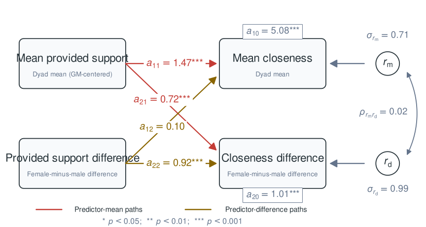
Fitted cross-sectional DSM for the example data. The nodes identify the mean and difference scores; edge and intercept labels show the estimated DSM coefficients, and the residual labels show the estimated score-component standard deviations and correlation.
The fixed effects from our MLM model map directly to these paths as such:
| Long-format fixed effect | DSM SEM path and interpretation |
|---|---|
| Intercept | : expected dyad-average closeness at the sample-average provided-support level and no female-male support difference |
| Provided-support dyad mean | : predictor level outcome level |
| Provided-support difference | : predictor difference outcome level |
| DSM role contrast | : expected female-minus-male outcome difference at the predictor reference values |
| Dyad mean role contrast | : predictor level outcome difference |
| Provided-support difference role contrast | : predictor difference outcome difference |
Thus, for example, is the change in dyad-average closeness associated with a one-unit larger female-minus-male provided-support difference, holding support level constant. In contrast, is the change in the female-minus-male closeness difference associated with that same one-unit larger support difference, holding support level constant. The and coefficients are the DSM cross-paths. They are omitted from the reduced DSM but are needed for the full model.
The random intercept variance is unexplained variance in outcome level, and the random role-contrast slope variance is unexplained variance in the full directional outcome difference. Their covariance indicates whether unexplained outcome level and unexplained outcome difference are associated.
The curved arrow is the scale-free correlation between the outcome-mean residual and the outcome-difference residual. It is not the female-male residual correlation from the APIM.
The DSM uses the full female-minus-male difference:
Therefore, this relationship applies:
For this reason, a nonzero indicates that the two roles have different residual variances. The remaining covariance between the partners’ residuals is
Reversing the coding
Instead of computing , we can reverse the direction and compute . This changes the direction of the differences, but not the substantive model.
cross_dsm_data_inverted <- dyadMLM::prepare_dyad_data(
  dyads_cross,
  dyad = coupleID,
  member = personID,
  role = gender,
  predictors = provided_support,
  # Request APIM columns too for comparison below.
  model_types = c("dsm", "apim"),
  add_apim_gmc_predictors = TRUE,
  keep_compositions = "female-male",
  dsm_role_order = c("male", "female")
)
dsm_model_inverted <- glmmTMB::glmmTMB(
  closeness ~
    .provided_support_dyad_mean_gmc +
    .provided_support_within_dyad_diff +
    .dsm_role_contrast +
    .provided_support_dyad_mean_gmc:.dsm_role_contrast +
    .provided_support_within_dyad_diff:.dsm_role_contrast +
    us(1 + .dsm_role_contrast | coupleID),
  dispformula = ~ 0,
  family = gaussian(),
  data = cross_dsm_data_inverted
)

female_minus_male <- glmmTMB::fixef(dsm_model)$cond
male_minus_female <- glmmTMB::fixef(dsm_model_inverted)$cond

knitr::kable(
  data.frame(
    `model term` = names(female_minus_male),
    `female - male` = unname(female_minus_male),
    `male - female` = unname(male_minus_female),
    check.names = FALSE
  ),
  digits = 3,
  align = c("l", "r", "r")
)| model term | female - male | male - female |
|---|---|---|
| (Intercept) | 5.097 | 5.097 |
| .provided_support_dyad_mean_gmc | 1.475 | 1.475 |
| .provided_support_within_dyad_diff | 0.107 | -0.107 |
| .dsm_role_contrast | 1.026 | -1.026 |
| .provided_support_dyad_mean_gmc:.dsm_role_contrast | 0.682 | -0.682 |
| .provided_support_within_dyad_diff:.dsm_role_contrast | 0.903 | 0.903 |
The two models have identical fitted values and model fit:
.provided_support_within_dyad_diffreverses because the predictor difference reverses..dsm_role_contrastreverses because the represented outcome difference reverses..provided_support_dyad_mean_gmc:.dsm_role_contrastreverses because only the outcome difference reverses..provided_support_within_dyad_diff:.dsm_role_contrastremains unchanged because both differences reverse.
The intercept and .provided_support_dyad_mean_gmc also
remain unchanged. For the random effects, the variances of
(Intercept) and .dsm_role_contrast remain
unchanged, whereas their covariance reverses sign.
Relationship to the APIM and DIM
For distinguishable dyads, the full DSM and an unconstrained distinguishable APIM are alternative parameterizations of the same fixed associations (Iida et al. 2018).
Let’s fit the equivalent distinguishable APIM:
apim_model <- glmmTMB::glmmTMB(
  closeness ~
    # Role-specific intercepts
    0 +
    .is_female +
    .is_male +

    # Role-specific actor effects
    .is_female:.provided_support_gmc_actor +
    .is_male:.provided_support_gmc_actor +

    # Role-specific partner effects
    .is_female:.provided_support_gmc_partner +
    .is_male:.provided_support_gmc_partner +

    # Role-specific Gaussian residual covariance structure
    us(0 +
         .is_female +
         .is_male
       | coupleID),
  dispformula = ~ 0,
  family = gaussian(),
  data = cross_dsm_data_inverted
)
The two DSM directions and the APIM have identical fit statistics:
data.frame(
  model = c("DSM: female - male", "DSM: male - female", "APIM"),
  AIC = round(c(AIC(dsm_model), AIC(dsm_model_inverted), AIC(apim_model)), 3),
  BIC = round(c(BIC(dsm_model), BIC(dsm_model_inverted), BIC(apim_model)), 3),
  logLik = round(c(
    as.numeric(logLik(dsm_model)),
    as.numeric(logLik(dsm_model_inverted)),
    as.numeric(logLik(apim_model))
  ), 3)
)
#>                model     AIC     BIC  logLik
#> 1 DSM: female - male 652.219 683.545 -317.11
#> 2 DSM: male - female 652.219 683.545 -317.11
#> 3               APIM 652.219 683.545 -317.11
Fixed-effect transformation
Let and denote the actor effects on the female and male outcomes. The corresponding partner effects are and , and the APIM intercepts are and . Fixed APIM coefficients use and write out their effect and outcome role. The numbered paths through retain the published DSM notation.
The slope transformation can be understood in two steps. First, for each outcome role , form the actor-plus-partner and actor-minus-partner combinations:
The DSM slopes then follow by combining the female- and male-outcome effects:
With complete pairs, the GMC APIM and DSM share a zero point, so the intercepts transform as
Raw APIM predictors leave the slope transformations unchanged but require intercept recentering.
For the reverse slope transformation, first recover the role-specific actor-plus-partner and actor-minus-partner combinations:
Then, for each outcome role ,
The intercepts transform back as
The following comparison applies the APIM-to-DSM transformation to all six fixed effects:
| DSM path | From APIM transformation | From DSM model |
|---|---|---|
| a10 | 5.097 | 5.097 |
| a11 | 1.475 | 1.475 |
| a12 | 0.107 | 0.107 |
| a20 | 1.026 | 1.026 |
| a21 | 0.682 | 0.682 |
| a22 | 0.903 | 0.903 |
Random-effect transformation
Let and be the APIM random effects for the female and male outcomes. The DSM outcome-level and outcome-difference residuals are the same random effects expressed in different coordinates:
Applying this rotation to the APIM covariance matrix reproduces the DSM random intercept variance, intercept-slope covariance, and role-slope variance:
apim_vcov <- as.matrix(glmmTMB::VarCorr(apim_model)$cond$coupleID)
dsm_vcov <- as.matrix(glmmTMB::VarCorr(dsm_model)$cond$coupleID)

rotation <- rbind(
  outcome_level = c(0.5, 0.5),
  outcome_difference = c(1, -1)
)
apim_to_dsm_vcov <- rotation %*% apim_vcov %*% t(rotation)

data.frame(
  parameter = c(
    "Var(outcome mean)",
    "Cov(outcome mean, outcome diff)",
    "Var(outcome diff)"
  ),
  from_DSM = round(c(
    dsm_vcov[1, 1],
    dsm_vcov[1, 2],
    dsm_vcov[2, 2]
  ), 3),
  from_APIM_transformation = round(c(
    apim_to_dsm_vcov[1, 1],
    apim_to_dsm_vcov[1, 2],
    apim_to_dsm_vcov[2, 2]
  ), 3)
)
#>                         parameter from_DSM from_APIM_transformation
#> 1               Var(outcome mean)    0.561                    0.561
#> 2 Cov(outcome mean, outcome diff)    0.029                    0.029
#> 3               Var(outcome diff)    1.208                    1.208
For exchangeable dyads, the direction of a member difference is
arbitrary. The directional intercept, both cross-paths, and the
covariance between outcome level and outcome difference must then be
zero. The remaining reduced, label-invariant DSM is algebraically the
Gaussian Dyad-Individual Model (DIM). In dyadMLM, use
model_types = "dim" for this exchangeable model and reserve
model_types = "dsm" for distinguishable dyads.
Because the Gaussian DIM is the exchangeability-constrained version of the full DSM, exchangeability can also be tested by comparing these nested models. This is equivalent to the comparison shown in Testing distinguishability in the APIM vignette.
Checking partner dependence
We can check whether the fitted DSM reproduces each role’s response variance and the partner correlation by comparing observed and simulated data.
dsm_simulations <- dyadMLM::simulate_dyad_responses(dsm_model, seed = 123)
dyadMLM::check_partner_dependence(
  dsm_simulations,
  dyad = coupleID,
  role = gender,
  # Supply the fitting data because gender is not in the model formula.
  data = cross_dsm_data
)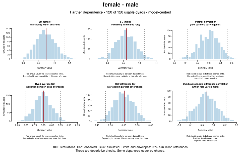
The top row shows role-specific SDs and partner correlation. The bottom row shows the same information using dyad averages and half the differences between partners. Histograms show simulated values and red lines mark observed values. A red line far from most simulations suggests a mismatch.
By default, the check subtracts the model’s fixed-effect predictions
from observed and simulated responses. Good agreement is often expected
for variances and correlations estimated from the same data. See the function
help for details and interpretation. Simulation studies show how
often the check detects omitted
partner dependence and incorrect
covariance pooling, and how often it raises false alarms. For
intensive longitudinal data, also supply member and
time. A separate
study covers this case.
The same dsm_simulations can be checked with check_dyad_residuals()
and check_dyad_outcomes(),
as shown in the APIM
vignette.
Intensive longitudinal DSM
The intensive longitudinal DSM extends the cross-sectional DSM using the same temporal decomposition and multilevel workflow shown for the intensive longitudinal DIM. The DSM retains the directional mean-and-difference parameterization described above. For more detail on centering decisions and mean-and-deviation interpretation, refer to the DIM vignette. For dynamic models and their cautions, see the dynamic ILD APIM example.
Brief example of ILD DSM:
ild_dsm_data <- dyadMLM::prepare_dyad_data(
  dyads_ild,
  dyad = coupleID,
  member = personID,
  role = gender,
  time = diaryday,
  predictors = provided_support,
  model_types = "dsm",
  keep_compositions = "female-male",
  dsm_role_order = c("female", "male")
)

print(ild_dsm_data, n = 4)
#> # dyadMLM data
#> # Rows: 3360 | Dyads: 120 | Intensive longitudinal: yes
#> # Structure: dyad = coupleID, member = personID, role = gender, time = diaryday
#> # DSM direction: female - male
#> #
#> # Dyad compositions:
#> # female_x_male distinguishable 120 dyads
#> #
#> # Added columns:
#> #   .composition                  inferred dyad composition
#> #   .composition_role             composition-specific member role
#> #   .is_{role}                    composition-role indicator columns
#> #   .{pred}_cwp                   within-person predictor: momentary deviations
#> #                                 from each person's usual level
#> #   .{pred}_cbp                   between-person predictor: stable differences
#> #                                 from the average person's usual level
#> #   .dsm_role_contrast            DSM role contrast: +0.5 for the first
#> #                                 declared role and -0.5 for the second
#> #                                 declared role
#> #   .{pred}_dyad_mean_gmc         dyad-mean predictor: dyad's average predictor
#> #                                 level, grand-mean centered
#> #   .{pred}_within_dyad_diff      DSM signed predictor difference: first
#> #                                 declared role minus second declared role
#> #   .{pred}_cwp_dyad_mean         within-person dyad-mean predictor: shared
#> #                                 momentary deviations in the dyad
#> #   .{pred}_cwp_within_dyad_diff  DSM within-person signed predictor
#> #                                 difference: first declared role minus second
#> #                                 declared role
#> #   .{pred}_cbp_dyad_mean         between-person dyad-mean predictor: dyad's
#> #                                 stable usual level, grand-mean centered
#> #   .{pred}_cbp_within_dyad_diff  DSM between-person signed predictor
#> #                                 difference: first declared role minus second
#> #                                 declared role
#> #
#> # A tibble: 3,360 × 19
#>   personID coupleID diaryday gender closeness provided_support .composition
#>      <int>    <int>    <int> <fct>      <dbl>            <dbl> <fct>
#> 1        1        1        0 female      3.74             4.93 female_x_male
#> 2        2        1        0 male        5.91             5.59 female_x_male
#> 3        1        1        1 female      3.72             4.89 female_x_male
#> 4        2        1        1 male        6.32             5.18 female_x_male
#> # ℹ 3,356 more rows
#> # ℹ 12 more variables: .composition_role <fct>, .is_female <dbl>,
#> #   .is_male <dbl>, .provided_support_cwp <dbl>, .provided_support_cbp <dbl>,
#> #   .dsm_role_contrast <dbl>, .provided_support_dyad_mean_gmc <dbl>,
#> #   .provided_support_cwp_dyad_mean <dbl>,
#> #   .provided_support_cbp_dyad_mean <dbl>,
#> #   .provided_support_within_dyad_diff <dbl>, …
The specification below estimates same-day associations between support and closeness and allows separate linear trends for the outcome level and the female-minus-male outcome difference. It also includes the role-specific AR(1) components specified and interpreted in the APIM vignette.
dsm_ILD <- glmmTMB::glmmTMB(
  closeness ~

    # Outcome-level intercept and linear time trend
    1 +
    diaryday +

    # Within-person predictor level -> outcome level
    .provided_support_cwp_dyad_mean +

    # Within-person predictor difference -> outcome level
    .provided_support_cwp_within_dyad_diff +

    # Between-person predictor level -> outcome level
    .provided_support_cbp_dyad_mean +

    # Between-person predictor difference -> outcome level
    .provided_support_cbp_within_dyad_diff +

    # Outcome-difference intercept and linear time trend
    .dsm_role_contrast +
    diaryday:.dsm_role_contrast +

    # Within-person predictor level and difference -> outcome difference
    .provided_support_cwp_dyad_mean:.dsm_role_contrast +
    .provided_support_cwp_within_dyad_diff:.dsm_role_contrast +

    # Between-person predictor level and difference -> outcome difference
    .provided_support_cbp_dyad_mean:.dsm_role_contrast +
    .provided_support_cbp_within_dyad_diff:.dsm_role_contrast +

    # Stable outcome-level and outcome-difference covariance
    us(1 + .dsm_role_contrast | coupleID) +

    # Same-day outcome-level and outcome-difference covariance
    us(1 + .dsm_role_contrast | coupleID:diaryday) +

    # Role-specific residual persistence
    ar1(0 + .is_female:factor(diaryday) | coupleID) +
    ar1(0 + .is_male:factor(diaryday) | coupleID),
  dispformula = ~ 0,
  family = gaussian(),
  data = ild_dsm_data,
  # Non-default settings help this example converge.
  control = glmmTMB::glmmTMBControl(
    profile = TRUE,
    optimizer = stats::optim,
    optArgs = list(method = "BFGS")
  )
)

glmmTMB::VarCorr(dsm_ILD)
#>
#> Conditional model:
#>  Groups            Name                         Std.Dev. Corr
#>  coupleID          (Intercept)                  0.70187
#>                    .dsm_role_contrast           0.99250  0.072
#>  coupleID.diaryday (Intercept)                  0.65167
#>                    .dsm_role_contrast           1.00690  0.022
#>  coupleID.1        .is_female:factor(diaryday)0 0.49444  0.592 (ar1)
#>  coupleID.2        .is_male:factor(diaryday)0   0.57571  0.658 (ar1)
This AR-adjusted, fixed-slope DSM omits the actor random slopes present in the simulation. See the distinguishable APIM AR(1) section for the corresponding specification and interpretation.
The cross-sectional path interpretation therefore applies separately at the within-person and between-person levels. At each level, the predictor dyad mean and directional difference predict both the outcome level and the directional outcome difference.
Return to the Actor-Partner Interdependence Model vignette, see the Dyad-Individual Model vignette for a related model specification, or return to the online package overview.