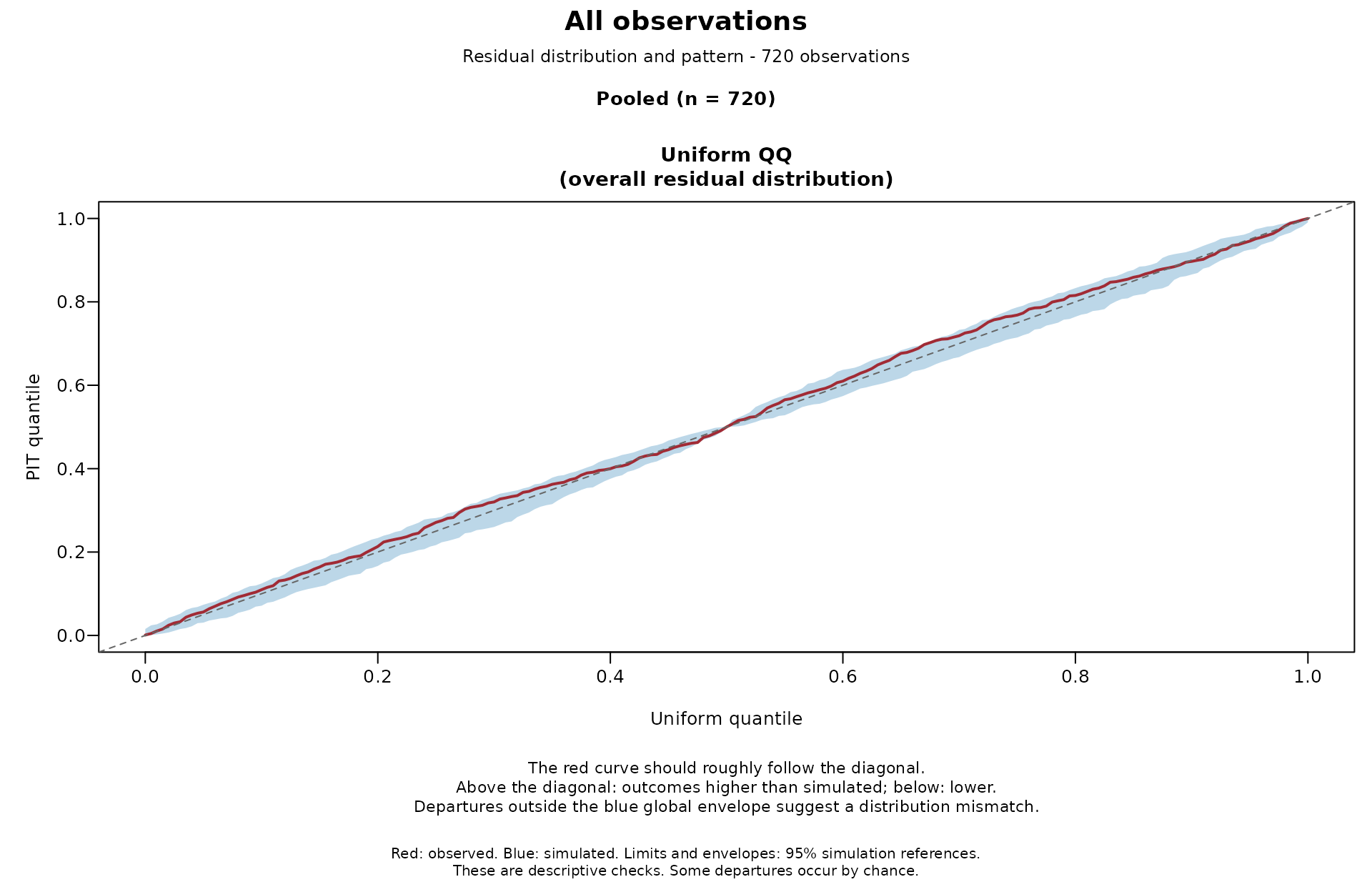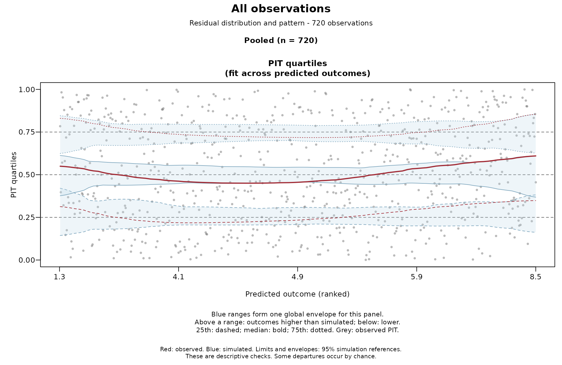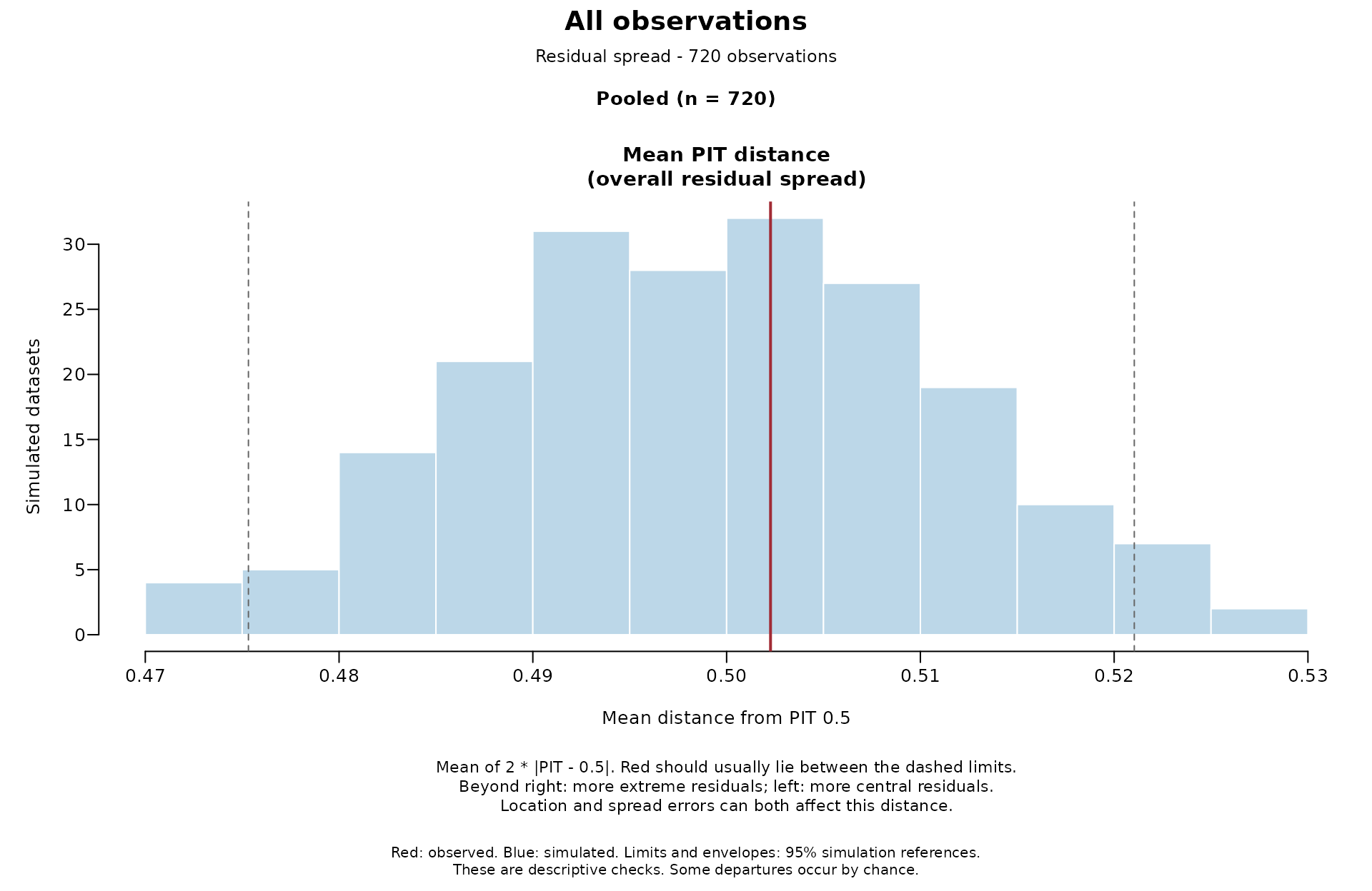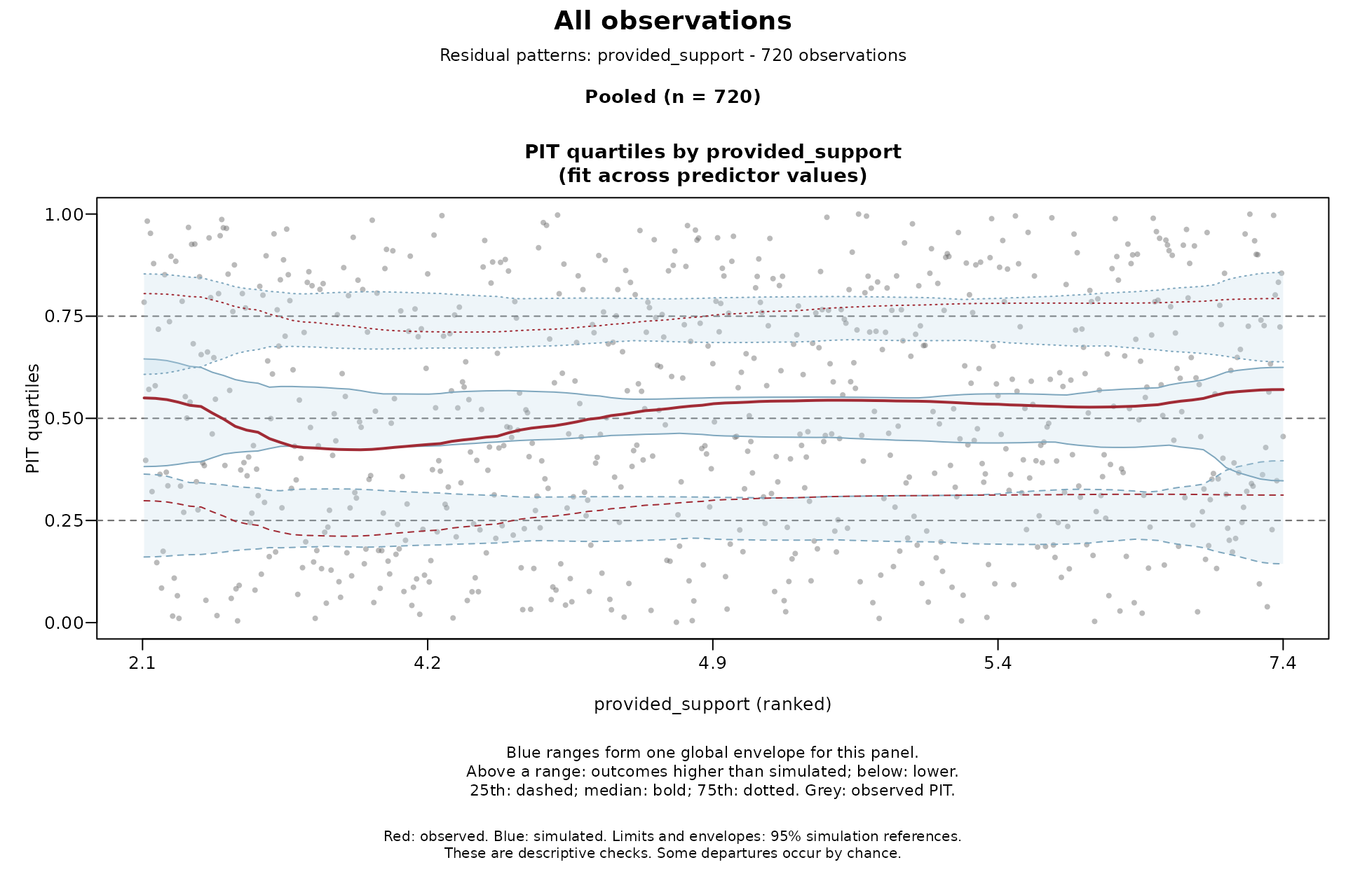
Check residual distributions and patterns
Source:R/predictive_checks_residuals.R
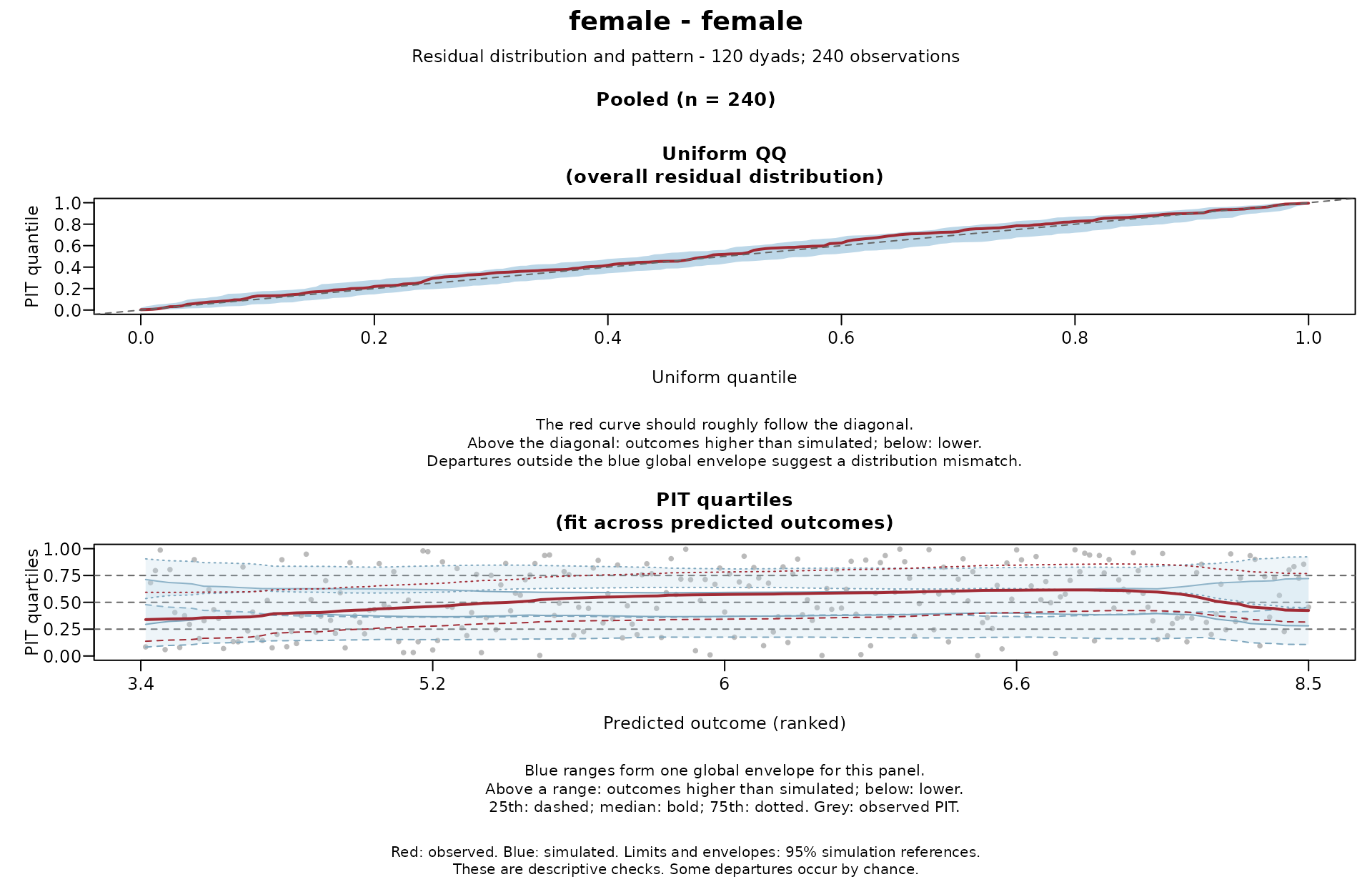
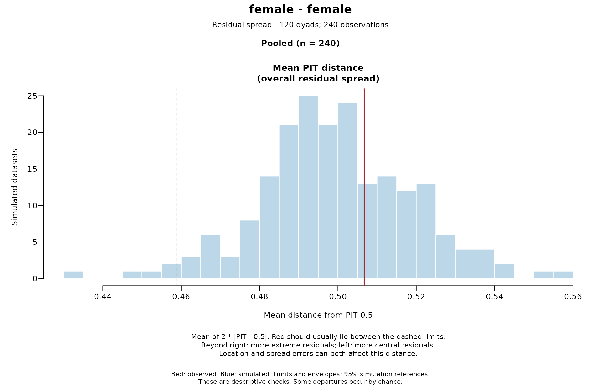
check_dyad_residuals.Rd A model should reproduce how responses are distributed around its
predictions. This check finds where each observed outcome falls among its
simulated values (PIT residuals), using complete datasets from
simulate_dyad_responses(). This helps identify mismatches in the model's
assumptions, such as the distribution family, dispersion, or predictor
effects.
For checks on the outcome scale, also run check_dyad_outcomes() with the
same simulations.
For guidance on how to read the plots, see plot.dyadMLM_residual_check().
Usage
check_dyad_residuals(
  simulations,
  dyad = NULL,
  role = NULL,
  member = NULL,
  predictors = NULL,
  seed = 123,
  plot = TRUE,
  ask = NULL,
  panels = TRUE,
  data = NULL,
  quartile_lines = c("bins", "qgam")
)
Arguments
- simulations
An object from
simulate_dyad_responses()with at least 200 simulated datasets. At least 1,000 are recommended for stable comparisons.- dyad
Dyad ID column, with or without quotes. Required when
roleis supplied.- role
Role column, with or without quotes, such as gender.
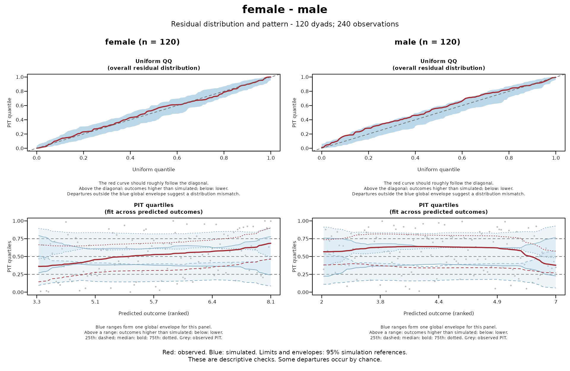
NULL(default) pools all observations. Otherwise, each composition (pair of partners' roles, such as female-male) is checked separately. Each member must keep the same role. With few dyads in a composition, the simulated ranges are wide, so its panels lack sensitivity.- member
Person ID column, with or without quotes. Required with
rolewhen dyads have repeated observations.- predictors
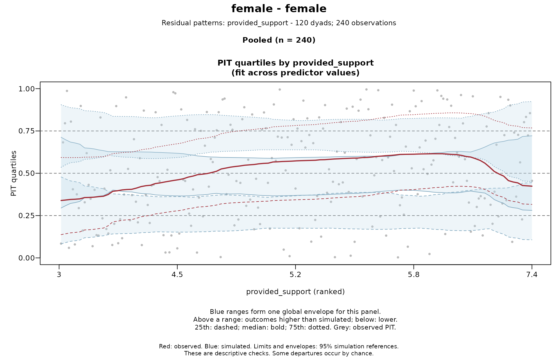
Optional quoted column names, e.g.
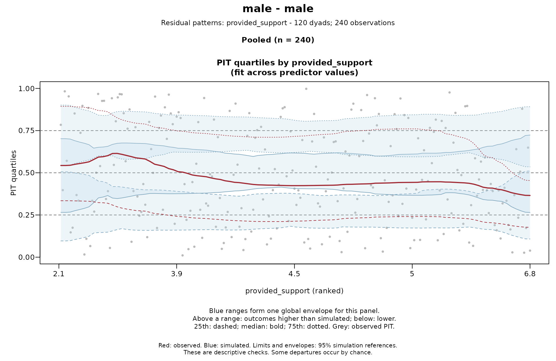
c("age", "stress"). Each adds a page of PIT quartiles across that column, to show effects the model omits or may misspecify, especially partner effects. Missing or infinite values are left out of that page only.NULL(default) adds no predictor pages.- seed
Seed for randomized PIT residuals. The caller's random-number state is restored afterwards. With
NULL, use and advance the caller's random-number state.- plot
If
TRUE(default), draw the comparison plots for visual checks. IfFALSE,askandpanelsare ignored.- ask
Whether to pause between figures on an interactive device.
NULL(default) pauses when there is more than one figure,TRUEpauses andFALSEdraws without pausing. File devices never pause.- panels
If
TRUE(default), arrange checks in figures by composition, with one column per role or a pooled column. IfFALSE, draw each check and role separately.- data
The unchanged data used to fit the model. Supply it when the columns you name (such as
role) are not in the model formulas. Also supply it when rows were excluded during fitting (e.g., for missing values). Otherwise, a person whose partner's rows were excluded has an unknown composition and is omitted.- quartile_lines
Quantile regression lines (
"qgam") can show trends near the ends of a numeric axis more clearly than smoothed bins ("bins", default). As in DHARMa, they are fitted with the qgam package (Fasiolo et al., 2021) and drawn on ranks of the axis values. Each dataset gets its own lines. Tuning qgam for every dataset would take far too long, so simulated datasets reuse the tuning chosen for the observed data. The 95% coverage of the qgam envelopes is therefore approximate."qgam"is much slower and may warn when fits do not converge.
Value
Invisibly returns a dyadMLM_residual_check list with the pit matrix
(after any centring) and calculated summaries in compositions. pit has
one row per fitted observation and one column per dataset (observed first,
then all simulated). Optionally, suppress plotting with plot = FALSE and
draw the saved result later with plot(result), which also takes ask and
panels.
Scope
Complete simulated datasets keep the fitted partner and time dependence and
any modeled differences in variability between roles. Unlike DHARMa's default
(since version 0.5.0), simulations redraw all random effects. Dyadic models
often fix the residual variance near zero (dispformula = ~ 0) and model the
partners' residual variances and covariance as random effects. If held
fixed, these random effects would reproduce the data almost exactly.
Parameters stay fixed at their fitted values, so parameter uncertainty is not
included. These are descriptive checks, not significance tests, and
differ from DHARMa's plots and tests (see the
distribution-checks article).
They do not directly assess serial correlation.
Predicted outcomes are mean predictions with random effects set to zero (see
simulate_dyad_responses()). The checks use the same fitted rows and
families as simulate_dyad_responses() and weight all observations equally.
For cross-sectional data, check partner correlations with
check_partner_dependence().
Method and credit
The internal calculation follows the simulation-based PIT approach used in Florian Hartig's DHARMa package and the randomized quantile residual method of Dunn and Smyth (1996). We implement the definition directly and keep the uniform 0–1 scale.
At each fitted row, rank the observed and all simulated outcomes together,
breaking ties randomly. For rank r among m datasets, use (r - U) / m,
where U is uniform between 0 and 1.
When the model freely estimates an overall location (an intercept or separate role means) and is not ordinal, PIT is centred automatically: each dataset's PIT is transformed to normal scores, centred on its median across all fitted rows, and transformed back. Panels then show residuals relative to this overall location, so all panels can show less of an overall shift. Centring also partly offsets how fitting makes departures look smaller.
Global envelopes use extreme-rank-length ordering (Myllymäki et al., 2017).
References
Dunn, P. K., & Smyth, G. K. (1996). Randomized quantile residuals. Journal of Computational and Graphical Statistics, 5(3), 236–244. doi:10.2307/1390802
Fasiolo, M., Wood, S. N., Zaffran, M., Nedellec, R., & Goude, Y. (2021). qgam: Bayesian nonparametric quantile regression modeling in R. Journal of Statistical Software, 100(9), 1–31. doi:10.18637/jss.v100.i09
Hartig, F. (2026). DHARMa: Residual diagnostics for hierarchical (multi-level/mixed) regression models (Version 0.5.0) [R package]. doi:10.32614/CRAN.package.DHARMa
Myllymäki, M., Mrkvička, T., Grabarnik, P., Seijo, H., & Hahn, U. (2017). Global envelope tests for spatial processes. Journal of the Royal Statistical Society: Series B (Statistical Methodology), 79(2), 381–404. doi:10.1111/rssb.12172
Examples
example_data <- prepare_dyad_data(
dyads_cross,
dyad = coupleID,
member = personID,
model_types = "none",
seed = 123
)
# Exchangeable dyads: the two random-effect blocks represent the partners'
# residual variances and covariance.
model <- glmmTMB::glmmTMB(
closeness ~ gender + provided_support +
us(1 | coupleID) + us(0 + .member_contrast_arbitrary | coupleID),
dispformula = ~ 0,
data = example_data
)
simulations <- simulate_dyad_responses(
model,
nsim = 200, # Low for a quick example. Use at least 1,000.
seed = 123
)
check_dyad_residuals(
simulations,
dyad = coupleID,
role = gender,
predictors = "provided_support",
ask = FALSE
)
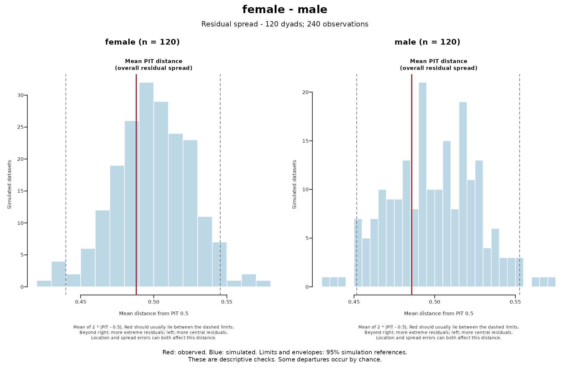
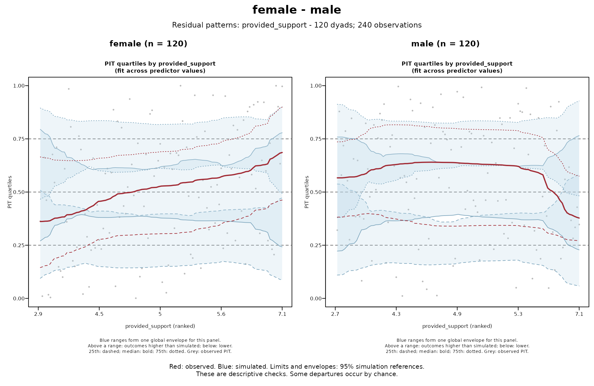
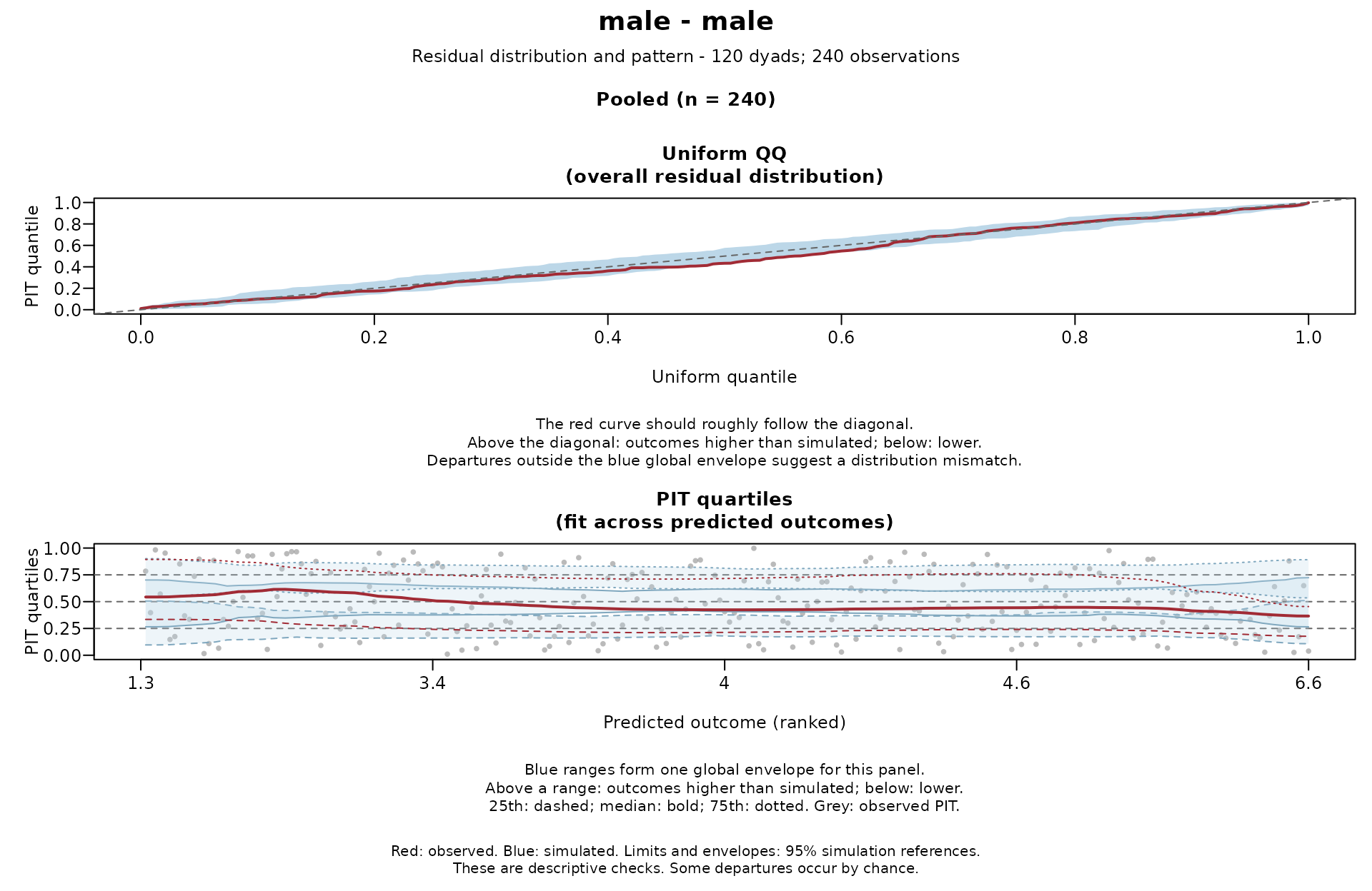
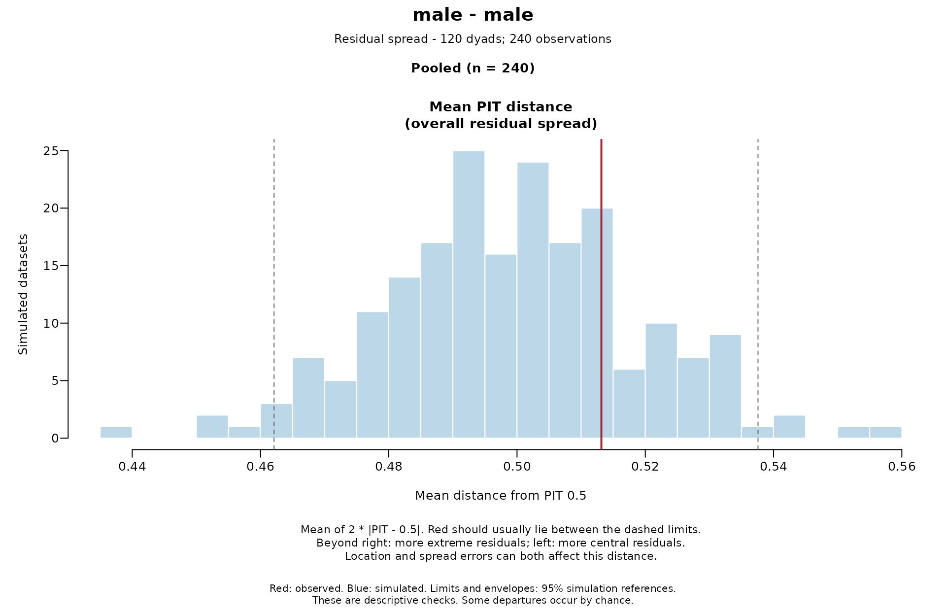
 # Save a pooled check without drawing, then plot each figure separately.
result <- check_dyad_residuals(
simulations,
role = NULL,
predictors = "provided_support",
plot = FALSE
)
plot(result, panels = FALSE, ask = FALSE)