
Check whether a fitted model reproduces partner dependence
Source:R/predictive_checks_dependence.R
check_partner_dependence.Rd![[Experimental]](figures/lifecycle-experimental.svg) A dyadic model should reproduce how much responses vary and how strongly
partners' responses are related. This check computes variances and correlations
of simulated responses based on the model and compares them to the observed
response variances and correlations from the data.
This helps identify mismatches in the model's assumptions. The check
currently supports cross-sectional dyads only (one response per partner).
A dyadic model should reproduce how much responses vary and how strongly
partners' responses are related. This check computes variances and correlations
of simulated responses based on the model and compares them to the observed
response variances and correlations from the data.
This helps identify mismatches in the model's assumptions. The check
currently supports cross-sectional dyads only (one response per partner).
Usage
check_partner_dependence(
  simulations,
  dyad,
  role = NULL,
  plot = TRUE,
  response = c("model-centred", "raw"),
  ask = NULL,
  panels = TRUE,
  data = NULL
)
Arguments
- simulations
An object returned by
simulate_dyad_responses().- dyad
The dyad column name. Looked up first in the fitted model frame, then in
dataif supplied.- role
The role column name. Looked up first in the fitted model frame, then in
dataif supplied.NULL(default) pools all dyads as exchangeable. Supply roles even for an exchangeable model to reveal variance or partner-correlation mismatches that pooling may hide. Each dyad composition (role pair, such as female-male) is checked separately, using exchangeable summaries for same-role pairs and role-specific summaries otherwise.- plot
If
TRUE(default), draw the comparison plots for visual checks. IfFALSE,askandpanelsare ignored.- response
"model-centred"(default) subtracts the same model predictions from observed and simulated responses. The predictive check then assesses whether the model reproduces the variance and partner correlations remaining after accounting for its fixed-effect predictions. This includes random effects and observation-level noise. With"raw", the predictive check assesses whether the full model, including fixed effects, reproduces the overall response variances and partner correlations. Seesimulate_dyad_responses()for how predictions are defined.- ask
Whether to pause between figures on an interactive device.
NULL(default) pauses when there is more than one figure,TRUEpauses andFALSEdraws without pausing. In panel mode, each composition is one figure. File devices never pause.- panels
If
TRUE(default), show each composition in one figure, with two rows and up to three columns. IfFALSE, draw each statistic separately. Graphics settings are restored afterwards.- data
Optional: the unchanged data frame used to fit the model. Supply it when
dyadorroleis not in the model formulas.
Value
The comparison plots (shown by default) are the main output. The
function invisibly returns a dyadMLM_partner_check object containing the
compositions table with pair counts and a statistics tibble for each
composition. Compositions with fewer than three complete dyads are skipped
and have NULL statistics. Each tibble has one observed row
followed by one row per simulation, identified by dataset. summary
compares each observed statistic with the middle 95% of its simulations
(lower, upper) and marks those outside it. The object includes
omission counts and settings, and can be saved and plotted later.
Reading the plots
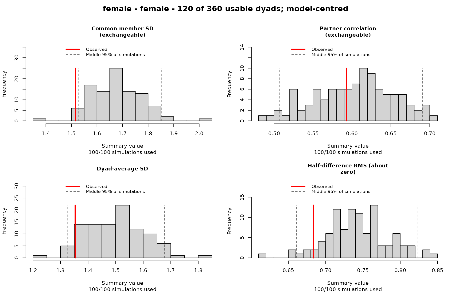
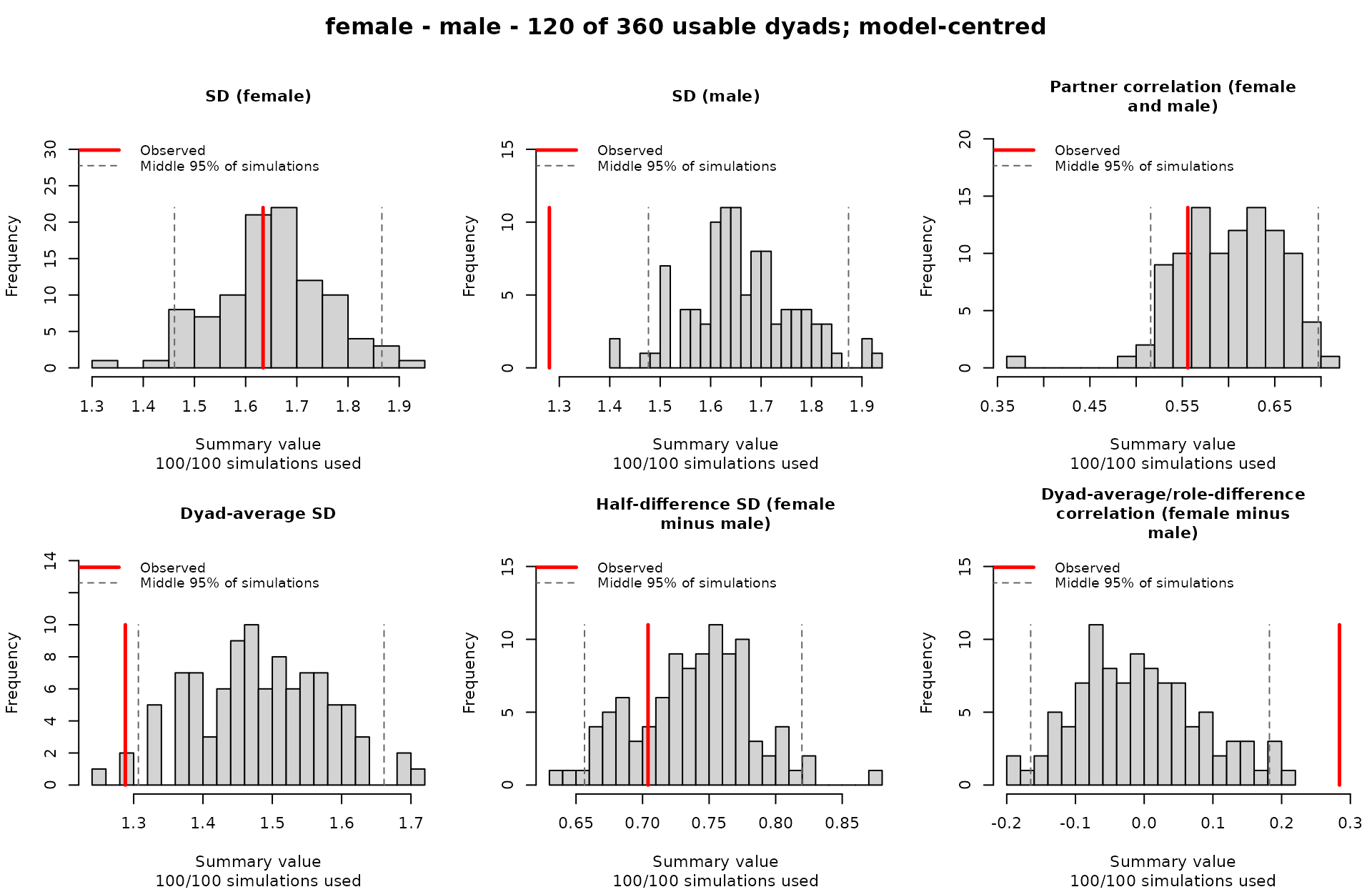
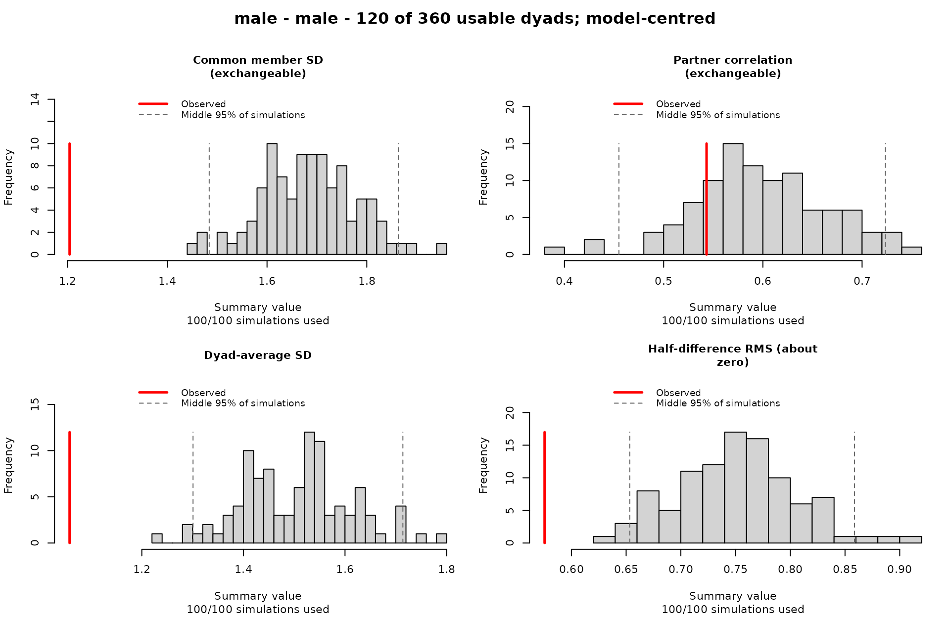
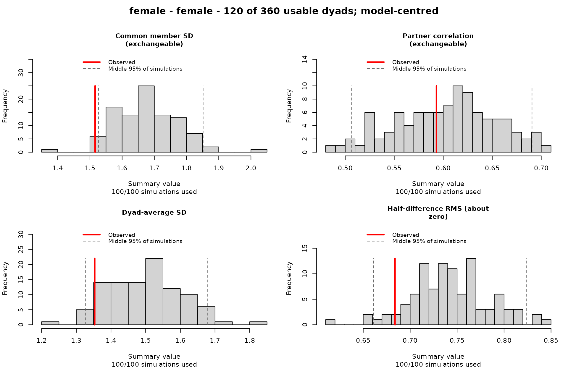
Histograms show simulated summaries. Red lines mark observed values. Dashed lines enclose the middle 95% of simulations (no formal confidence intervals). The heading shows the dyad composition, its number of usable dyads, and the total across all compositions. The top row shows member SDs and partner correlation. The bottom row shows the same information using dyad averages and partner differences.
An observed value far from most simulated values may indicate that the model does not reproduce that feature of the data well. Agreement does not establish that omitted dependence is negligible, especially with few dyads. The partner-dependence study illustrates how sample size affects detection when residual partner correlation is omitted.
Checking each composition can reveal differences hidden by pooling.
Flags (observed values outside the middle 95%, marked * when printed) can
occur by chance, especially when checking several summaries.
They invite investigation, not formal rejection of the model. The
covariance-pooling study
illustrates detection and false alarms when checking each composition; 10 to
29% of correctly pooled models had at least one flag.
The top row compares:
Response SDs: one for each role, or one common SD for exchangeable members.
Partner correlation: how strongly partners' responses are related.
The bottom row shows:
Dyad-average SD: how much dyads differ in their average response.
Half-difference SD or RMS: each partner difference is divided by two. With distinct roles, the SD shows how much signed differences vary across dyads. For exchangeable members, the RMS (root mean square) shows their typical size, regardless of partner order.
Dyad-average/role-difference correlation: shown only for distinct roles, because it depends on how partners are ordered. Positive values indicate greater variance for the first named role. Negative values indicate greater variance for the second.
These checks are particularly useful when a less restricted model does not converge and so cannot be used for model comparison. They show how well the simpler model reproduces the observed variances and partner correlations.
A flexible covariance model will usually reproduce features it estimated from
the same data. Agreement alone therefore does not establish good fit.
For example, pooled summaries (role = NULL) of a Gaussian model with an
unconstrained exchangeable covariance, as below, agree almost by construction.
Use a suitable model comparison to formally test a specific covariance
restriction when both models can be fitted (see compare_nested_models()).
Rows with missing IDs or roles and incomplete dyads are omitted with a warning.
Technical details
After any centring, paired responses a and b are used to compute
dyad averages M = (a + b) / 2 and half-differences D = (a - b) / 2.
Roles follow factor levels or sorted values.
For exchangeable members, common member variance is var(M) + mean(D^2) and
partner covariance is var(M) - mean(D^2). Partner correlation is
covariance divided by variance. Half-difference RMS is sqrt(mean(D^2)).
The variance and covariance calculations for exchangeable dyads follow Woody and Sadler (2005).
References
Woody, E., & Sadler, P. (2005). Structural equation models for interchangeable dyads: Being the same makes a difference. Psychological Methods, 10(2), 139-158. doi:10.1037/1082-989X.10.2.139 .
Gelman, A., Meng, X.-L., & Stern, H. S. (1996). Posterior predictive assessment of model fitness via realized discrepancies. Statistica Sinica, 6, 733-807.
Examples
# Data contains three compositions: female-female, female-male, and male-male.
example_data <- prepare_dyad_data(
dyads_cross,
dyad = coupleID,
member = personID,
model_types = "none",
seed = 123
)
# This model pools all compositions and treats every dyad as exchangeable.
model <- glmmTMB::glmmTMB(
closeness ~ 1 +
us(1 | coupleID) +
us(0 + .member_contrast_arbitrary | coupleID),
dispformula = ~ 0,
data = example_data
)
# Fewer simulations for a quick example (the default is 1000).
simulations <- simulate_dyad_responses(
model,
nsim = 100,
seed = 123
)
check_partner_dependence(
simulations,
dyad = coupleID,
role = gender,
# Supply the fitting data because gender is not in the model formula.
data = example_data
)
 # Optionally, suppress plot, store object, and plot later.
check <- check_partner_dependence(
simulations,
dyad = coupleID,
role = gender,
data = example_data,
plot = FALSE
)
# Check how well the model reproduces variances and partner correlations
# within each dyad composition.
plot(check, ask = FALSE, panels = TRUE)
# Optionally, suppress plot, store object, and plot later.
check <- check_partner_dependence(
simulations,
dyad = coupleID,
role = gender,
data = example_data,
plot = FALSE
)
# Check how well the model reproduces variances and partner correlations
# within each dyad composition.
plot(check, ask = FALSE, panels = TRUE)
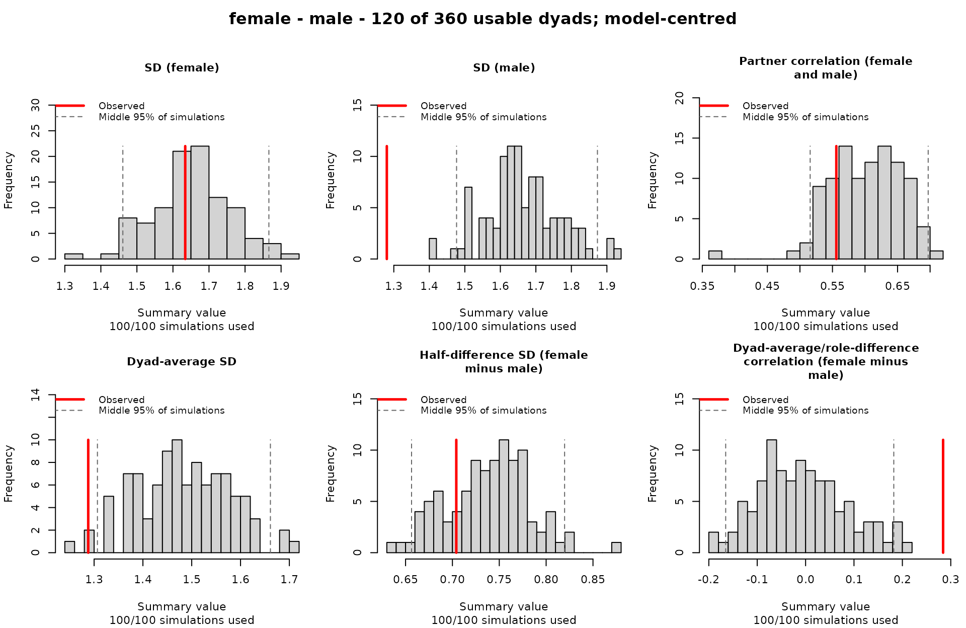
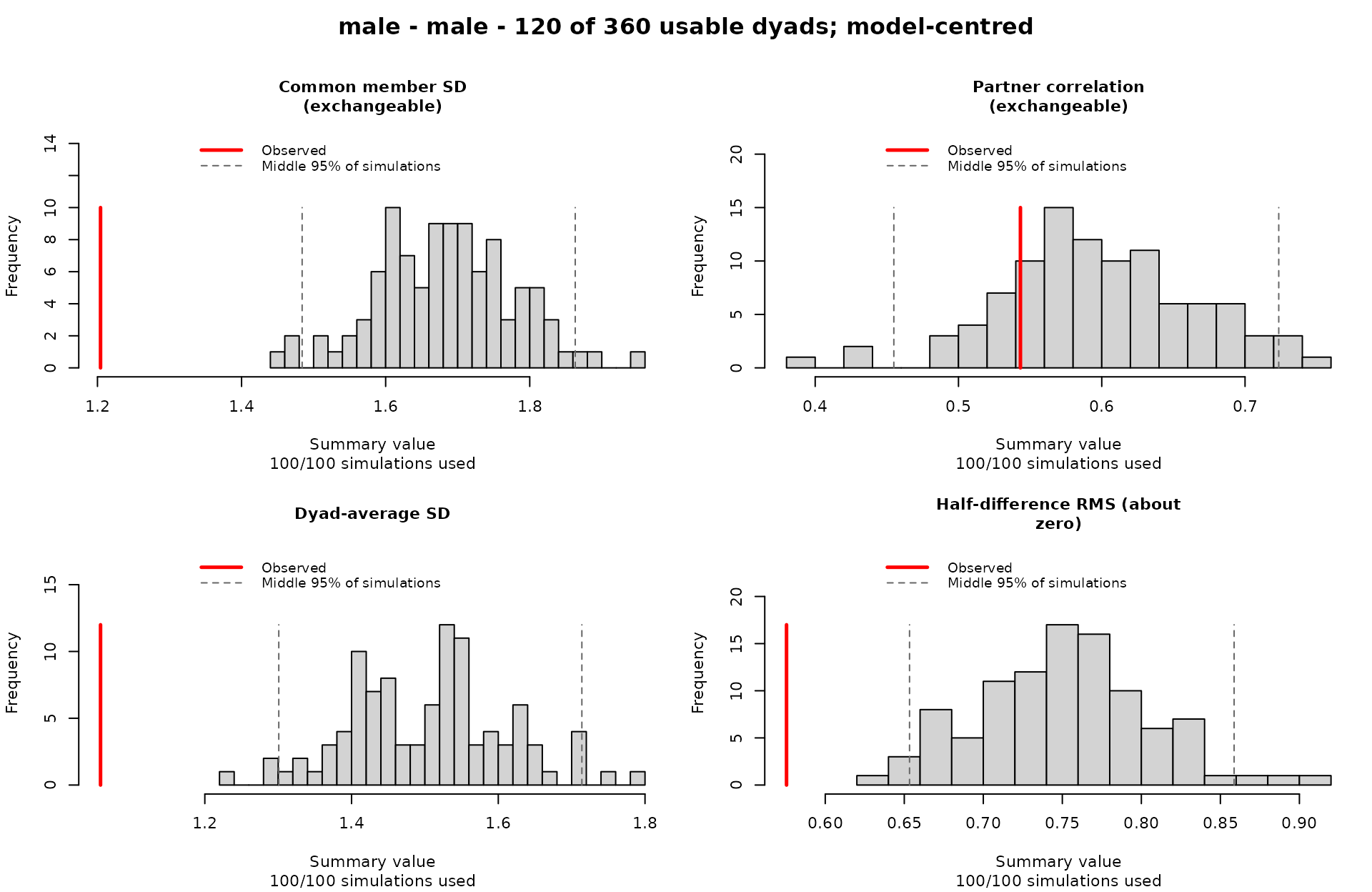 # Composition checks flag differences that the pooled check misses.
print(check)
#> <dyadMLM partner-dependence check>
#> Response: model-centred
#> Reference: 100 plug-in predictive datasets with new random effects
#>
#> female - female: 120 of 360 usable dyads
#> Observed 2.5% 97.5% Statistic
#> 1.516 1.527 1.851 * Common member SD (exchangeable)
#> 0.593 0.507 0.691 Partner correlation (exchangeable)
#> 1.353 1.326 1.678 Dyad-average SD
#> 0.684 0.661 0.824 Half-difference RMS (about zero)
#>
#> female - male: 120 of 360 usable dyads
#> Observed 2.5% 97.5% Statistic
#> 1.634 1.461 1.866 SD (female)
#> 1.280 1.477 1.873 * SD (male)
#> 0.556 0.516 0.697 Partner correlation (female and male)
#> 1.288 1.307 1.661 * Dyad-average SD
#> 0.704 0.656 0.820 Half-difference SD (female minus male)
#> 0.284 -0.165 0.182 * Dyad-average/role-difference correlation (female minus male)
#>
#> male - male: 120 of 360 usable dyads
#> Observed 2.5% 97.5% Statistic
#> 1.204 1.484 1.863 * Common member SD (exchangeable)
#> 0.543 0.455 0.724 Partner correlation (exchangeable)
#> 1.058 1.301 1.714 * Dyad-average SD
#> 0.576 0.653 0.859 * Half-difference RMS (about zero)
#>
#> Outside the middle 95% of simulations (*): 7 of 14 observed statistics.
#> Some departures occur by chance; these are descriptive checks, not significance tests.
#> Use plot(x) to view the comparisons.
# Composition checks flag differences that the pooled check misses.
print(check)
#> <dyadMLM partner-dependence check>
#> Response: model-centred
#> Reference: 100 plug-in predictive datasets with new random effects
#>
#> female - female: 120 of 360 usable dyads
#> Observed 2.5% 97.5% Statistic
#> 1.516 1.527 1.851 * Common member SD (exchangeable)
#> 0.593 0.507 0.691 Partner correlation (exchangeable)
#> 1.353 1.326 1.678 Dyad-average SD
#> 0.684 0.661 0.824 Half-difference RMS (about zero)
#>
#> female - male: 120 of 360 usable dyads
#> Observed 2.5% 97.5% Statistic
#> 1.634 1.461 1.866 SD (female)
#> 1.280 1.477 1.873 * SD (male)
#> 0.556 0.516 0.697 Partner correlation (female and male)
#> 1.288 1.307 1.661 * Dyad-average SD
#> 0.704 0.656 0.820 Half-difference SD (female minus male)
#> 0.284 -0.165 0.182 * Dyad-average/role-difference correlation (female minus male)
#>
#> male - male: 120 of 360 usable dyads
#> Observed 2.5% 97.5% Statistic
#> 1.204 1.484 1.863 * Common member SD (exchangeable)
#> 0.543 0.455 0.724 Partner correlation (exchangeable)
#> 1.058 1.301 1.714 * Dyad-average SD
#> 0.576 0.653 0.859 * Half-difference RMS (about zero)
#>
#> Outside the middle 95% of simulations (*): 7 of 14 observed statistics.
#> Some departures occur by chance; these are descriptive checks, not significance tests.
#> Use plot(x) to view the comparisons.