This vignette focuses on Gaussian cross-sectional and intensive longitudinal Actor-Partner Interdependence Models for distinguishable and exchangeable dyads. The intensive longitudinal examples cover concurrent associations, member-specific residual persistence, and a brief lagged-outcome extension.
For the broader package workflow and an overview of the available model-specific vignettes, including the Dyad-Individual Model and Dyadic Score Model, see the online package overview.
A vignette with non-Gaussian APIM examples is planned.
Cross-sectional APIMs
These examples use add_apim_gmc_predictors = TRUE, which
retains raw APIM columns and adds variants centered over all retained
non-missing source values. Using raw columns instead changes only the
intercept reference. Do not include both variants in a model with an
intercept.
The distinguishable APIM
A conceptual example for distinguishable female-male dyads:
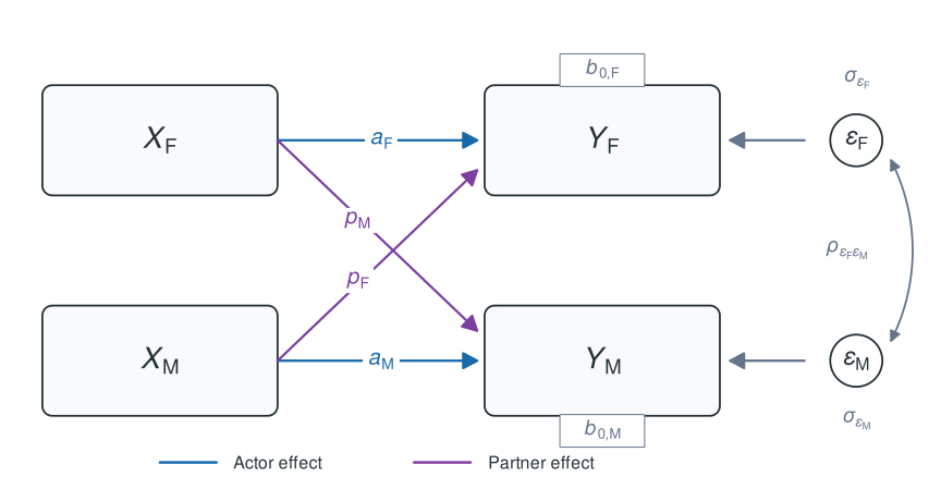
Conceptual cross-sectional APIM for distinguishable female-male dyads, with both predictors centered using one pooled grand mean. Intercepts , actor effects , and partner effects can differ by the role of the outcome member (F and M), and the two outcome residuals covary within dyads.
For univariate MLM software like glmmTMB, this model is
fitted in long format with one outcome row per member, which can be
visualized as:
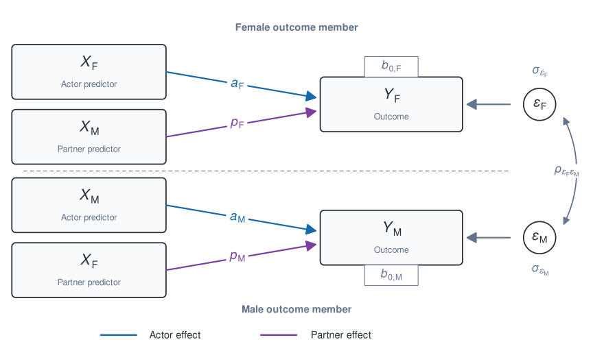
Individual-level representation of the distinguishable cross-sectional APIM used for the long-format multilevel model. Both predictors use one pooled grand-mean reference. For the female outcome, the female predictor is the actor predictor and the male predictor is the partner predictor. These roles reverse for the male outcome. Intercepts, actor coefficients, and partner coefficients may differ by outcome role, and the two member residuals may have different variances and covary.
Residual random-effects structure
For a distinguishable female-male dyad, the two members can have different residual variances. In the notation below, the member role is written first and indexes dyads. The within-dyad residual covariance block (shared across dyads) is:
And the full residual covariance matrix for all dyads (first three shown) is then block-diagonal:
This structure is estimated with an unstructured random-effects block
such as us(0 + .is_female + .is_male | coupleID) and
dispformula = ~ 0.
Fitting the distinguishable APIM with glmmTMB
We first prepare the example data with
dyadMLM::prepare_dyad_data():
apim_distinguishable_data <- dyadMLM::prepare_dyad_data(
  data = dyads_cross,
  dyad = coupleID,
  member = personID,
  role = gender,
  predictors = provided_support,
  model_types = "apim",
  add_apim_gmc_predictors = TRUE,
  # All three observed compositions in `dyads_cross` are detected and retained by
  # default. This example focuses on `female-male` dyads, so we restrict the
  # analysis here.
  keep_compositions = "female-male",
  include_arbitrary_member_contrast = TRUE,
  seed = 123
)

print(apim_distinguishable_data, n=4)
#> # dyadMLM data
#> # Rows: 240 | Dyads: 120 | Intensive longitudinal: no
#> # Structure: dyad = coupleID, member = personID, role = gender
#> #
#> # Dyad compositions:
#> # female_x_male distinguishable 120 dyads
#> #
#> # Added columns:
#> #   .composition                inferred dyad composition
#> #   .composition_role           composition-specific member role
#> #   .is_{role}                  composition-role indicator columns
#> #   .member_contrast_arbitrary  composition-specific member contrasts coded
#> #                               -1/+1 in arbitrary direction for
#> #                               exchangeability-constrained random effects.
#> #                               Values are 0 for other compositions
#> #   .{pred}_actor               APIM actor predictor: actor's original
#> #                               predictor values
#> #   .{pred}_partner             APIM partner predictor: partner's original
#> #                               predictor values
#> #   .{pred}_gmc                 APIM grand-mean-centered predictor source:
#> #                               original values minus the mean across all
#> #                               retained non-missing observations
#> #   .{pred}_gmc_actor           APIM grand-mean-centered actor predictor:
#> #                               actor's value relative to the mean across all
#> #                               retained non-missing observations
#> #   .{pred}_gmc_partner         APIM grand-mean-centered partner predictor:
#> #                               partner's value relative to the mean across all
#> #                               retained non-missing observations
#> #
#> # A tibble: 240 × 15
#>   personID coupleID gender closeness provided_support .composition
#>      <int>    <int> <fct>      <dbl>            <dbl> <fct>
#> 1        1        1 female      4.71             4.49 female_x_male
#> 2        2        1 male        4.61             4.76 female_x_male
#> 3        3        2 female      6.69             4.09 female_x_male
#> 4        4        2 male        5.98             6.20 female_x_male
#> # ℹ 236 more rows
#> # ℹ 9 more variables: .composition_role <fct>, .is_female <dbl>,
#> #   .is_male <dbl>, .member_contrast_arbitrary <dbl>,
#> #   .provided_support_gmc <dbl>, .provided_support_actor <dbl>,
#> #   .provided_support_partner <dbl>, .provided_support_gmc_actor <dbl>,
#> #   .provided_support_gmc_partner <dbl>
The optional member contrast is used later for the restricted model. It does not change the composition’s distinguishable metadata or role indicators.
apim_distinguishable_model <- glmmTMB::glmmTMB(
  closeness ~

    # Gender-specific intercepts
    0 +
    .is_female +
    .is_male +

    # Gender-specific actor effects
    .is_female:.provided_support_gmc_actor +
    .is_male:.provided_support_gmc_actor +

    # Gender-specific partner effects
    .is_female:.provided_support_gmc_partner +
    .is_male:.provided_support_gmc_partner +

    # Dyad-level unstructured random effects represent the two partner
    # residual variances and their covariance when dispformula = ~ 0.
    # This is glmmTMB-specific syntax! `brms` uses different syntax.
    us(0 +
         .is_female +
         .is_male
       | coupleID)

  , dispformula = ~ 0
  , family = gaussian()
  , data = apim_distinguishable_data
)

summary(apim_distinguishable_model)
#>  Family: gaussian  ( identity )
#> Formula:
#> closeness ~ 0 + .is_female + .is_male + .is_female:.provided_support_gmc_actor +
#>     .is_male:.provided_support_gmc_actor + .is_female:.provided_support_gmc_partner +
#>     .is_male:.provided_support_gmc_partner + us(0 + .is_female +
#>     .is_male | coupleID)
#> Dispersion:                 ~0
#> Data: apim_distinguishable_data
#>
#>       AIC       BIC    logLik -2*log(L)  df.resid
#>     652.2     683.5    -317.1     634.2       231
#>
#> Random effects:
#>
#> Conditional model:
#>  Groups   Name       Variance Std.Dev. Corr
#>  coupleID .is_female 0.8916   0.9442
#>           .is_male   0.8343   0.9134   0.30
#> Number of obs: 240, groups:  coupleID, 120
#>
#> Conditional model:
#>                                          Estimate Std. Error z value Pr(>|z|)
#> .is_female                                5.61050    0.08860   63.32  < 2e-16
#> .is_male                                  4.58410    0.08571   53.48  < 2e-16
#> .is_female:.provided_support_gmc_actor    1.46654    0.12321   11.90  < 2e-16
#> .is_male:.provided_support_gmc_actor      0.91142    0.10777    8.46  < 2e-16
#> .is_female:.provided_support_gmc_partner  0.34944    0.11141    3.14  0.00171
#> .is_male:.provided_support_gmc_partner    0.22226    0.11918    1.86  0.06219
#>
#> .is_female                               ***
#> .is_male                                 ***
#> .is_female:.provided_support_gmc_actor   ***
#> .is_male:.provided_support_gmc_actor     ***
#> .is_female:.provided_support_gmc_partner **
#> .is_male:.provided_support_gmc_partner   .
#> ---
#> Signif. codes:  0 '***' 0.001 '**' 0.01 '*' 0.05 '.' 0.1 ' ' 1
With the common centering, the two intercepts are the expected female and male closeness scores when both partners’ provided support equals the pooled sample mean. The estimated coefficients map as follows:
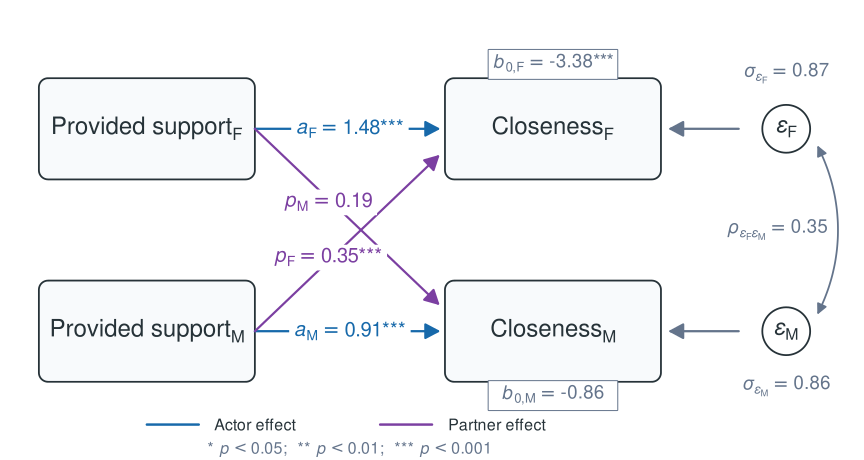
Fitted cross-sectional distinguishable APIM for the example data. Fixed effects, residual standard deviations, and the residual correlation are extracted from the fitted model.
The exchangeable APIM
Conceptually, the exchangeable APIM constrains several of the effects to be equal:
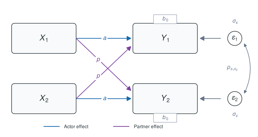
Conceptual cross-sectional APIM for exchangeable dyads, with both predictors centered using one pooled grand mean. The two members share one intercept, one actor effect, and one partner effect. Their outcome residuals have equal variances, yet still covary within dyads.
Because the member labels are arbitrary, swapping members 1 and 2 does not change the model.
To estimate this model in a univariate MLM framework, we can draw a conceptual diagram as such:
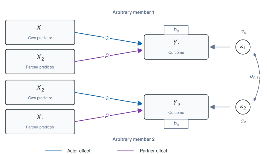
Individual-level representation of the exchangeable cross-sectional APIM used for the long-format multilevel model. Both predictors use one pooled grand-mean reference. The members share the same intercept. Each member’s own predictor has the shared actor effect, and the other member’s predictor has the shared partner effect. The two residual variances are equal and the residuals may covary.
Modeling the residual random-effects structure
For a simple random-intercept structure, equal member variances and their covariance can be specified directly. The specification becomes more difficult when the same exchangeability constraints must cover several random slopes. A single homogeneous structure would impose one variance across intercepts and slopes, whereas separate structures would omit their correlations.
The shared/difference representation works for residuals and other
random-effect terms, including random slopes. Following del Rosario and West (2025),
dyadMLM::prepare_dyad_data() generates an arbitrary
member-difference column, named .member_contrast_*. This
contrast is +1 for one member and -1 for the
other. The exchangeable residual structure is represented by two
separate random-effects terms: a shared dyad random intercept and a
random coefficient for this difference column. Additional random slopes
can be included in both blocks without changing this logic.
We fit a simple exchangeable APIM and then use
dyadMLM::recover_exchangeable_covariance() to
back-transform its shared/difference representation into a member-level
residual covariance matrix.
Fitting the restricted exchangeable APIM with glmmTMB
The restricted model omits gender-specific fixed effects and uses the
shared/difference residual representation. We reuse
apim_distinguishable_data, so both models use exactly the
same prepared rows and centering.
set_exchangeable_compositions would instead reclassify the
composition when it should be treated as exchangeable throughout an
analysis.
We then use the columns to fit the model as follows:
apim_exchangeable_model <- glmmTMB::glmmTMB(
  closeness ~

    # Pooled single intercept
    1 +

    # Pooled single actor and partner effects
    .provided_support_gmc_actor +
    .provided_support_gmc_partner +

    # Residual variance covariance matrix via the shared/difference
    # specification in two uncorrelated blocks
    us(1 | coupleID) +
    us(0 + .member_contrast_arbitrary | coupleID),
  dispformula = ~ 0,
  family = gaussian(),
  data = apim_distinguishable_data
)

summary(apim_exchangeable_model)
#>  Family: gaussian  ( identity )
#> Formula:
#> closeness ~ 1 + .provided_support_gmc_actor + .provided_support_gmc_partner +
#>     us(1 | coupleID) + us(0 + .member_contrast_arbitrary | coupleID)
#> Dispersion:                 ~0
#> Data: apim_distinguishable_data
#>
#>       AIC       BIC    logLik -2*log(L)  df.resid
#>     731.7     749.1    -360.8     721.7       235
#>
#> Random effects:
#>
#> Conditional model:
#>  Groups     Name                       Variance Std.Dev.
#>  coupleID   (Intercept)                0.5695   0.7547
#>  coupleID.1 .member_contrast_arbitrary 0.6156   0.7846
#> Number of obs: 240, groups:  coupleID, 120
#>
#> Conditional model:
#>                               Estimate Std. Error z value Pr(>|z|)
#> (Intercept)                    5.11917    0.06889   74.31   <2e-16 ***
#> .provided_support_gmc_actor    1.28459    0.09408   13.65   <2e-16 ***
#> .provided_support_gmc_partner  0.17553    0.09408    1.87   0.0621 .
#> ---
#> Signif. codes:  0 '***' 0.001 '**' 0.01 '*' 0.05 '.' 0.1 ' ' 1
We use dyadMLM::recover_exchangeable_covariance() to
recover the interpretable variance-covariance matrix:
backtransformed <- dyadMLM::recover_exchangeable_covariance(apim_exchangeable_model)

# residual variance-covariance and SD-correlation representations
print(backtransformed)
#> Recovered exchangeable member-level covariance
#>
#> Pair `pair_1`
#> Shared:     us(1 | coupleID)
#> Difference: us(0 + .member_contrast_arbitrary | coupleID)
#>
#> Variance-covariance:
#>                        1      2
#> 1 member1: (Intercept) 1.185  -0.046
#> 2 member2: (Intercept) -0.046 1.185
#>
#> Standard deviations and correlations:
#>                        1      2
#> 1 member1: (Intercept) 1.089  -0.039
#> 2 member2: (Intercept) -0.039 1.089
The back-transformation follows directly from the shared and member-difference random effects. If is the shared effect for dyad and its member-difference effect, the two member effects are
Because the two fitted blocks are independent,
With the common centering, the shared intercept is the expected closeness of either member when both partners’ provided support equals the pooled sample mean. The output can now be mapped as follows:
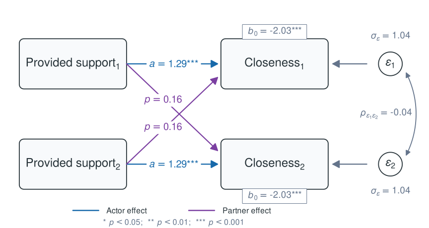
Fitted cross-sectional exchangeable APIM for the example data. The common member residual standard deviation and residual correlation are back-transformed from the fitted mean and difference components.
Testing distinguishability
Distinguishability can be evaluated by comparing a full model in which the two roles may differ with a restricted exchangeable model. This comparison tests the imposed equality constraints jointly. Here, they concern the fixed intercepts, actor effects, partner effects, and residual variances.
Both models use the same prepared data object. The full model uses its retained role indicators. The restricted model instead uses the opt-in arbitrary member contrast for the exchangeability-constrained residual structure.
dyadMLM::compare_nested_models() verifies that both
models use equivalent original observations before performing the
likelihood-ratio test:
dyadMLM::compare_nested_models(
  apim_exchangeable_model,
  apim_distinguishable_model
)
#> Likelihood-ratio test for nested models fitted to equivalent data
#> Assumes mathematical nesting and an appropriate chi-squared reference distribution.
#>
#>                            Df    AIC    BIC  logLik deviance  Chisq Chi Df
#> apim_exchangeable_model     5 731.67 749.07 -360.83   721.67
#> apim_distinguishable_model  9 652.22 683.55 -317.11   634.22 87.448      4
#>                            Pr(>Chisq)
#> apim_exchangeable_model
#> apim_distinguishable_model  < 2.2e-16 ***
#> ---
#> Signif. codes:  0 '***' 0.001 '**' 0.01 '*' 0.05 '.' 0.1 ' ' 1
#>
#> Conclusion (5% level): The likelihood-ratio test provides evidence that `apim_distinguishable_model` fits better than `apim_exchangeable_model` (p < 0.001).
The test provides evidence against all restrictions jointly, but it does not show which parameter differs. The helper also cannot determine whether the models are mathematically nested. That remains a modeling requirement. The usual chi-squared reference distribution may be unreliable when a tested variance parameter lies on its boundary.
Checking partner dependence
The model comparison tests the restrictions jointly. Predictive checks show whether the restricted model reproduces each role’s variance and the partner correlation. We supply the original roles to examine their variances separately.
apim_simulations <- dyadMLM::simulate_dyad_responses(
  apim_exchangeable_model, seed = 123
)
dyadMLM::check_partner_dependence(
  apim_simulations,
  dyad = coupleID,
  role = gender,
  # Supply the fitting data because gender is not in the model formula.
  data = apim_distinguishable_data
)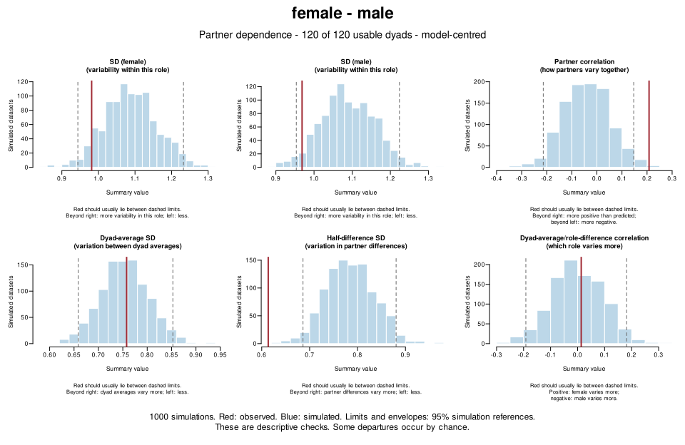
The top row shows role-specific SDs and partner correlation. The bottom row shows the same information using dyad averages and half the differences between partners. Histograms show simulated values and red lines mark observed values. A red line far from most simulations suggests a mismatch.
Here, the restricted model produces a lower partner correlation than observed. It also overstates how much the partner differences vary across dyads. The plots do not identify which restriction causes the mismatch.
By default, the check subtracts the model’s fixed-effect predictions
from observed and simulated responses. Good agreement is often expected
for variances and correlations estimated from the same data. See the function
help for details and interpretation. Simulation studies show how
often the check detects omitted
partner dependence and incorrect
covariance pooling, and how often it raises false alarms. For
intensive longitudinal data, also supply member and
time. A separate
study covers this case.
Checking residuals and outcomes
We reuse apim_simulations with check_dyad_residuals()
and check_dyad_outcomes().
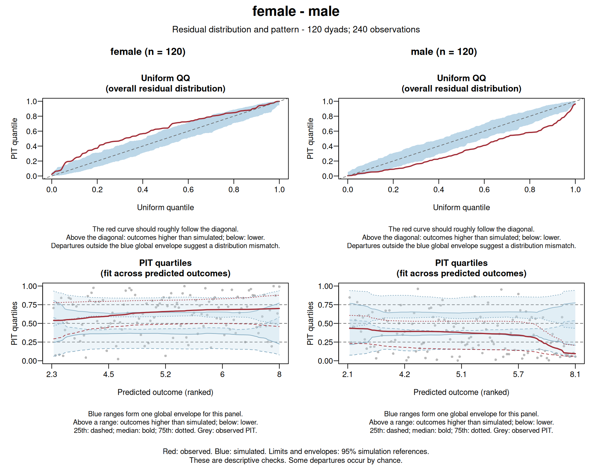
The residual check uses PIT residuals, which rank each outcome from 0
(low) to 1 (high) among its simulated values. The outcome check compares
outcome distributions and summaries.
We check by gender (role = gender), even though the
restricted model treats partners as exchangeable. We do this because
role differences the model misses can cancel out when all observations
are pooled: if one role’s outcomes are higher than simulated and the
other’s lower, a pooled check can look fine. Here, the pooled QQ plot
(not shown) stays inside its envelope. Any other column that gives each
member a fixed role, such as older and younger partner, can be checked
the same way.
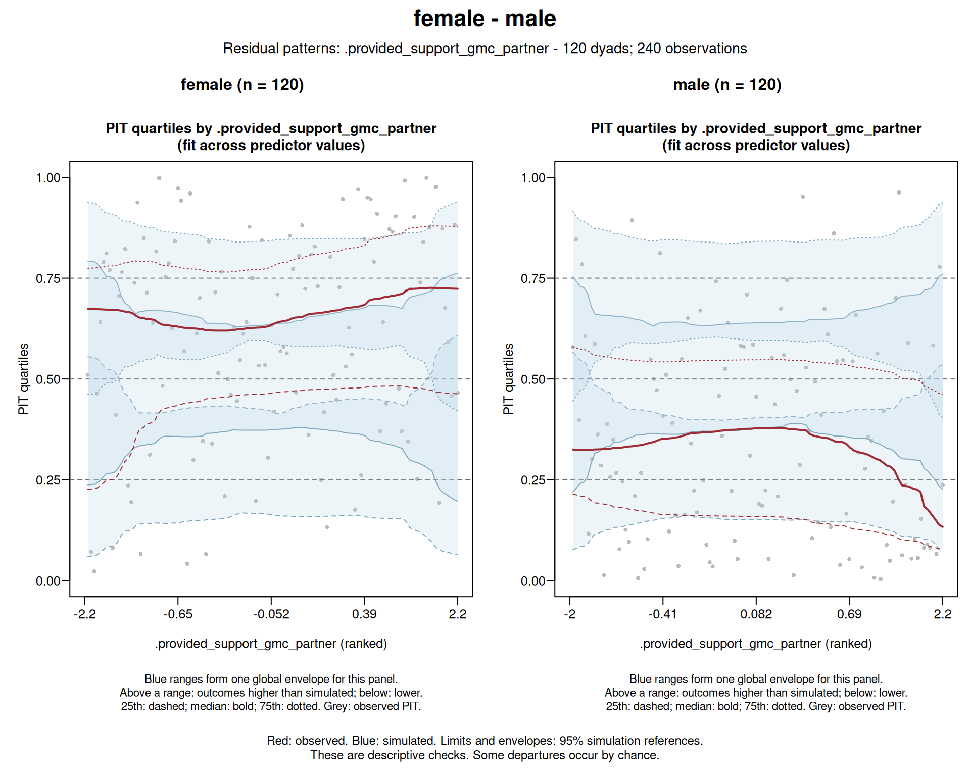
With predictors, we add a page of PIT quartiles across
the partner’s provided support. If the model captures the partner
effect, the quartiles stay near their dashed lines at 0.25, 0.5, and
0.75 for all levels of partner support. With a missing or misspecified
partner effect, they move away from these lines as partner support
changes.
dyadMLM::check_dyad_residuals(
  apim_simulations,
  dyad = coupleID,
  role = gender,
  predictors = ".provided_support_gmc_partner",
  data = apim_distinguishable_data
)
dyadMLM::check_dyad_outcomes(
  apim_simulations,
  dyad = coupleID,
  role = gender,
  data = apim_distinguishable_data
)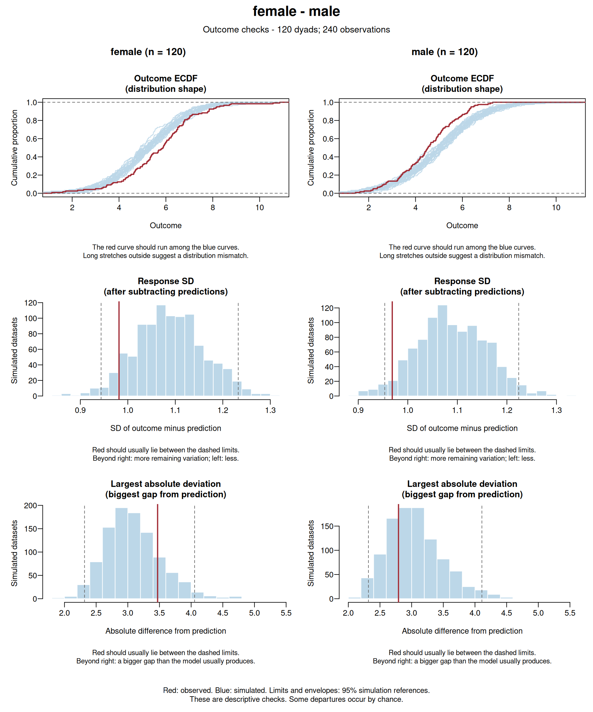
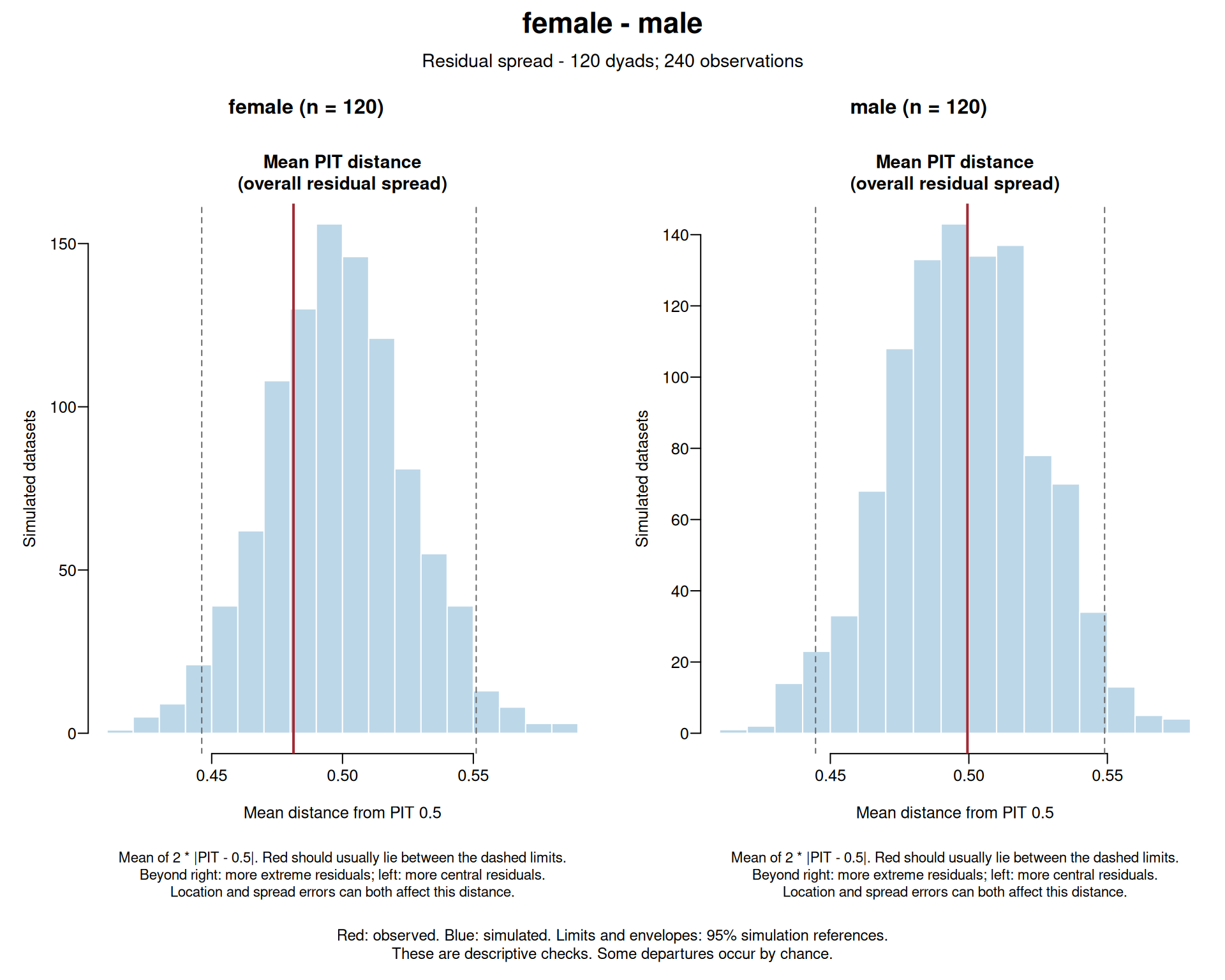
Look for flags (red curves outside their blue envelopes, or red lines outside their dashed limits) that form a pattern across plots. Here, women’s observed closeness is higher than simulated and men’s closeness is lower, in the QQ plots, the PIT quartiles, and the outcome ECDFs. For men, the gap grows at high predicted outcomes, as well as at high partner support. Mean PIT distance, response SDs, and largest absolute deviations stay within their limits. These panels mainly react to spread, so the model seems to reproduce how much closeness varies around its predictions. The pattern suggests that the model omits relevant gender differences, at least in mean closeness.
Adding gender-specific intercepts
(0 + .is_female + .is_male instead of 1) makes
the actor estimate smaller and the partner estimate larger. Women
provide slightly more support than men here, so the omitted gender
difference in mean closeness had shifted both effects. Rechecking this
model (not shown) flags only men’s PIT quartiles across predicted
outcomes. The distinguishable APIM, which also lets actor and partner
effects and residual variances differ by gender, shows no flags. The simulation
study shows how often these panels flag correct and mismatched
models.
If you know DHARMa: the uniform QQ plot and the PIT quartiles across predicted outcomes use the same principle as its residual plots and are read the same way. Two things differ:
- Our simulations redraw all random effects. DHARMa’s default (since
version 0.5.0) holds them at their fitted values and redraws only the
residual variation. In APIMs fitted with
dispformula = ~ 0, as here, the random effects absorb all residual variation, so these simulations would reproduce the data almost exactly. Redrawing all random effects also keeps partner dependence in the reference. - The blue envelopes are global envelopes (Myllymäki et al. 2017) built from whole simulated datasets, which keep the fitted partner and time dependence. They are an alternative to DHARMa’s tests, which assume independent residuals.
Intensive longitudinal APIMs
For longitudinal APIMs, time-varying predictors are decomposed into
within-person and between-person components before actor and partner
variables are constructed (Bolger and Laurenceau
2013; Gistelinck and Loeys 2020). The default "auto"
selects "2l" when both time and
predictors are supplied. The within-person
(cwp) component captures occasion-specific deviations from
each member’s observed mean, whereas the between-person
(cbp) component captures each member’s observed mean
relative to the sample grand mean.
Note that observed person means used to construct the between-person
(cbp) predictors can be unreliable when each member
contributes few occasions, which can bias
between-person estimates (Gottfredson
2019).
Concurrent ILD Gaussian APIM for distinguishable dyads
The decomposition above can be combined with role-specific effects. We first retain the female-male distinction when preparing the data:
ild_distinguishable_data <- dyadMLM::prepare_dyad_data(
  dyads_ild,
  dyad = coupleID,
  member = personID,
  role = gender,
  time = diaryday,
  predictors = provided_support,
  model_types = "apim",
  keep_compositions = "female-male"
) |>
  dplyr::mutate(
    # we grand-mean center in this example to help convergence and
    # interpretation
    diaryday_gmc = diaryday - mean(diaryday)
  )
The following model allows the intercepts, time trends, and within-
and between-person actor and partner effects to differ between female
and male members. Centering diaryday makes the
role-specific intercepts refer to the average study day:
ild_distinguishable_model <- glmmTMB::glmmTMB(
  closeness ~
    0 +

    # Role-specific intercepts
    .is_female +
    .is_male +

    # Role-specific time trends
    .is_female:diaryday_gmc +
    .is_male:diaryday_gmc +

    # Role-specific within-person actor effects
    .is_female:.provided_support_cwp_actor +
    .is_male:.provided_support_cwp_actor +

    # Role-specific within-person partner effects
    .is_female:.provided_support_cwp_partner +
    .is_male:.provided_support_cwp_partner +

    # Role-specific between-person actor effects
    .is_female:.provided_support_cbp_actor +
    .is_male:.provided_support_cbp_actor +

    # Role-specific between-person partner effects
    .is_female:.provided_support_cbp_partner +
    .is_male:.provided_support_cbp_partner +

    # Stable dyad-level covariance
    us(0 + .is_female + .is_male | coupleID) +

    # Same-occasion covariance
    us(0 + .is_female + .is_male |
         coupleID:diaryday),
  dispformula = ~ 0,
  family = gaussian(),
  data = ild_distinguishable_data
)
#> Warning in finalizeTMB(TMBStruc, obj, fit, h, data.tmb.old): Model convergence
#> problem; false convergence (8). See vignette('troubleshooting'),
#> help('diagnose')
Adding role-specific residual AR(1)
The same-occasion block above allows the partners’ residuals to covary within a day, but it does not describe persistence across days. In glmmTMB, we can model independent persistent AR(1) components per member.
For distinguishable dyads, we add one term for each role while retaining the same-occasion covariance. We spell out the complete model so the concurrent and persistent components are visible together.
ild_distinguishable_ar_model <- glmmTMB::glmmTMB(
  closeness ~
    0 +

    # Role-specific intercepts
    .is_female +
    .is_male +

    # Role-specific time trends
    .is_female:diaryday_gmc +
    .is_male:diaryday_gmc +

    # Role-specific within-person actor effects
    .is_female:.provided_support_cwp_actor +
    .is_male:.provided_support_cwp_actor +

    # Role-specific within-person partner effects
    .is_female:.provided_support_cwp_partner +
    .is_male:.provided_support_cwp_partner +

    # Role-specific between-person actor effects
    .is_female:.provided_support_cbp_actor +
    .is_male:.provided_support_cbp_actor +

    # Role-specific between-person partner effects
    .is_female:.provided_support_cbp_partner +
    .is_male:.provided_support_cbp_partner +

    # Stable dyad-level covariance
    us(0 + .is_female + .is_male | coupleID) +

    # Same-occasion covariance
    us(0 + .is_female + .is_male |
         coupleID:diaryday) +

    # Role-specific residual persistence
    ar1(0 + .is_female:factor(diaryday) | coupleID) +
    ar1(0 + .is_male:factor(diaryday) | coupleID),
  dispformula = ~ 0,
  family = gaussian(),
  data = ild_distinguishable_data,
  # Non-default settings help this example converge.
  control = glmmTMB::glmmTMBControl(profile = TRUE)
)

glmmTMB::VarCorr(ild_distinguishable_ar_model)
#>
#> Conditional model:
#>  Groups            Name                         Std.Dev. Corr
#>  coupleID          .is_female                   0.88813
#>                    .is_male                     0.83006  0.334
#>  coupleID.diaryday .is_female                   0.83204
#>                    .is_male                     0.81486  0.253
#>  coupleID.1        .is_female:factor(diaryday)0 0.49444  0.592 (ar1)
#>  coupleID.2        .is_male:factor(diaryday)0   0.57571  0.658 (ar1)
The two AR standard deviations and correlations describe each role’s persistent component. They are not correlations of the complete residual and do not represent partner influence. The dyad-day block continues to describe the remaining same-day variances and partner covariance.
Random slopes
For example, role-specific within-person actor random slopes can be added by replacing the stable dyad-level block above with:
us(
  0 +
    .is_female +
    .is_male +
    .is_female:.provided_support_cwp_actor +
    .is_male:.provided_support_cwp_actor
  | coupleID
)
This block estimates the covariance among the two role-specific random intercepts and actor slopes.
Concurrent ILD Gaussian APIM for exchangeable dyads
In longitudinal Gaussian exchangeable APIMs, the sum-and-difference parametrization from del Rosario and West (2025) can be extended to the dyad-occasion level to represent same-occasion residual dependence.
We first prepare within-person (cwp) and between-person
(cbp) actor and partner predictors. We retain the
female-female dyads as one substantively exchangeable composition:
ild_apim_data <- dyadMLM::prepare_dyad_data(
  dyads_ild,
  dyad = coupleID,
  member = personID,
  role = gender,
  time = diaryday,
  predictors = provided_support,
  model_types = "apim",
  keep_compositions = "female-female",
  seed = 123
)

print(ild_apim_data, n = 4)
#> # dyadMLM data
#> # Rows: 3360 | Dyads: 120 | Intensive longitudinal: yes
#> # Structure: dyad = coupleID, member = personID, role = gender, time = diaryday
#> #
#> # Dyad compositions:
#> # female_x_female exchangeable 120 dyads
#> #
#> # Added columns:
#> #   .composition                inferred dyad composition
#> #   .composition_role           composition-specific member role
#> #   .is_exchangeable            composition-role indicator columns
#> #   .member_contrast_arbitrary  composition-specific member contrasts coded
#> #                               -1/+1 in arbitrary direction for
#> #                               exchangeability-constrained random effects.
#> #                               Values are 0 for other compositions
#> #   .{pred}_cwp                 within-person predictor: momentary deviations
#> #                               from each person's usual level
#> #   .{pred}_cbp                 between-person predictor: stable differences
#> #                               from the average person's usual level
#> #   .{pred}_actor               APIM actor predictor: actor's original
#> #                               predictor values
#> #   .{pred}_partner             APIM partner predictor: partner's original
#> #                               predictor values
#> #   .{pred}_cwp_actor           APIM within-person actor predictor: actor's
#> #                               momentary deviations from their usual level
#> #   .{pred}_cwp_partner         APIM within-person partner predictor: partner's
#> #                               momentary deviations from their usual level
#> #   .{pred}_cbp_actor           APIM between-person actor predictor: actor's
#> #                               stable difference from the average person's
#> #                               usual level
#> #   .{pred}_cbp_partner         APIM between-person partner predictor:
#> #                               partner's stable difference from the average
#> #                               person's usual level
#> #
#> # A tibble: 3,360 × 18
#>   personID coupleID diaryday gender closeness provided_support .composition
#>      <int>    <int>    <int> <fct>      <dbl>            <dbl> <fct>
#> 1      241      121        0 female      6.60             6.18 female_x_female
#> 2      242      121        0 female      5.22             5.70 female_x_female
#> 3      241      121        1 female      8.33             4.57 female_x_female
#> 4      242      121        1 female      5.24             5.30 female_x_female
#> # ℹ 3,356 more rows
#> # ℹ 11 more variables: .composition_role <fct>, .is_exchangeable <dbl>,
#> #   .member_contrast_arbitrary <dbl>, .provided_support_cwp <dbl>,
#> #   .provided_support_cbp <dbl>, .provided_support_actor <dbl>,
#> #   .provided_support_partner <dbl>, .provided_support_cwp_actor <dbl>,
#> #   .provided_support_cwp_partner <dbl>, .provided_support_cbp_actor <dbl>,
#> #   .provided_support_cbp_partner <dbl>
The example below estimates same-day associations between support and
closeness and includes diaryday to adjust for a linear time
trend. Its stable and same-occasion covariance blocks impose
exchangeability through paired shared and member-contrast terms.
ild_apim_model <- glmmTMB::glmmTMB(
  closeness ~
    1 +

    diaryday +

    # Within-person actor and partner effects
    .provided_support_cwp_actor +
    .provided_support_cwp_partner +

    # Between-person actor and partner effects
    .provided_support_cbp_actor +
    .provided_support_cbp_partner +

    # Stable exchangeable dyad-level covariance
    us(1 | coupleID) +
    us(0 + .member_contrast_arbitrary | coupleID) +

    # Same-occasion exchangeable covariance
    us(1 | coupleID:diaryday) +
    us(0 + .member_contrast_arbitrary | coupleID:diaryday)

  , dispformula = ~ 0
  , family = gaussian()
  , data = ild_apim_data
)

summary(ild_apim_model)
#>  Family: gaussian  ( identity )
#> Formula:
#> closeness ~ 1 + diaryday + .provided_support_cwp_actor + .provided_support_cwp_partner +
#>     .provided_support_cbp_actor + .provided_support_cbp_partner +
#>     us(1 | coupleID) + us(0 + .member_contrast_arbitrary | coupleID) +
#>     us(1 | coupleID:diaryday) + us(0 + .member_contrast_arbitrary |
#>     coupleID:diaryday)
#> Dispersion:                 ~0
#> Data: ild_apim_data
#>
#>       AIC       BIC    logLik -2*log(L)  df.resid
#>    9901.1    9962.3   -4940.6    9881.1      3350
#>
#> Random effects:
#>
#> Conditional model:
#>  Groups              Name                       Variance Std.Dev.
#>  coupleID            (Intercept)                0.5372   0.7330
#>  coupleID.1          .member_contrast_arbitrary 0.3021   0.5496
#>  coupleID.diaryday   (Intercept)                0.5718   0.7561
#>  coupleID.diaryday.1 .member_contrast_arbitrary 0.3714   0.6094
#> Number of obs: 3360, groups:  coupleID, 120; coupleID:diaryday, 1680
#>
#> Conditional model:
#>                               Estimate Std. Error z value Pr(>|z|)
#> (Intercept)                   5.906484   0.075513   78.22  < 2e-16 ***
#> diaryday                      0.006260   0.004576    1.37    0.171
#> .provided_support_cwp_actor   0.236697   0.024720    9.58  < 2e-16 ***
#> .provided_support_cwp_partner 0.245028   0.024720    9.91  < 2e-16 ***
#> .provided_support_cbp_actor   1.198981   0.076545   15.66  < 2e-16 ***
#> .provided_support_cbp_partner 0.354490   0.076545    4.63 3.64e-06 ***
#> ---
#> Signif. codes:  0 '***' 0.001 '**' 0.01 '*' 0.05 '.' 0.1 ' ' 1
Adding pooled residual AR(1)
Under exchangeability, each member still has a separate time series, but the AR standard deviation and correlation are pooled. We add one term grouped by the member nested within the dyad:
ild_exchangeable_ar_model <- glmmTMB::glmmTMB(
  closeness ~
    1 +

    diaryday +

    # Within-person actor and partner effects
    .provided_support_cwp_actor +
    .provided_support_cwp_partner +

    # Between-person actor and partner effects
    .provided_support_cbp_actor +
    .provided_support_cbp_partner +

    # Stable exchangeable dyad-level covariance
    us(1 | coupleID) +
    us(0 + .member_contrast_arbitrary | coupleID) +

    # Same-occasion exchangeable covariance
    us(1 | coupleID:diaryday) +
    us(0 + .member_contrast_arbitrary | coupleID:diaryday) +

    # Pooled residual persistence across member series
    ar1(0 + factor(diaryday) | coupleID:personID),
  dispformula = ~ 0,
  family = gaussian(),
  data = ild_apim_data,
  # Non-default settings help this example converge.
  control = glmmTMB::glmmTMBControl(profile = TRUE)
)

glmmTMB::VarCorr(ild_exchangeable_ar_model)
#>
#> Conditional model:
#>  Groups              Name                       Std.Dev. Corr
#>  coupleID            (Intercept)                0.71486
#>  coupleID.1          .member_contrast_arbitrary 0.52485
#>  coupleID.diaryday   (Intercept)                0.67201
#>  coupleID.diaryday.1 .member_contrast_arbitrary 0.49488
#>  coupleID.personID   factor(diaryday)0          0.55221  0.598 (ar1)
The pooled AR parameters describe the persistent within-member component. The dyad-day blocks continue to describe same-day partner covariance.
For the fitted AR model, we can recover the member-level covariance matrices for both the stable dyad effects and the same-occasion residual dependence. The two matched block pairs are returned separately:
recovered_covariance <- dyadMLM::recover_exchangeable_covariance(
  ild_exchangeable_ar_model
)

print(recovered_covariance)
#> Recovered exchangeable member-level covariances (2 block pairs)
#>
#> Pair `pair_1`
#> Shared:     us(1 | coupleID)
#> Difference: us(0 + .member_contrast_arbitrary | coupleID)
#>
#> Variance-covariance:
#>                        1     2
#> 1 member1: (Intercept) 0.786 0.236
#> 2 member2: (Intercept) 0.236 0.786
#>
#> Standard deviations and correlations:
#>                        1     2
#> 1 member1: (Intercept) 0.887 0.300
#> 2 member2: (Intercept) 0.300 0.887
#>
#> Pair `pair_2`
#> Shared:     us(1 | coupleID:diaryday)
#> Difference: us(0 + .member_contrast_arbitrary | coupleID:diaryday)
#>
#> Variance-covariance:
#>                        1     2
#> 1 member1: (Intercept) 0.697 0.207
#> 2 member2: (Intercept) 0.207 0.697
#>
#> Standard deviations and correlations:
#>                        1     2
#> 1 member1: (Intercept) 0.835 0.297
#> 2 member2: (Intercept) 0.297 0.835
The cwp terms estimate actor and partner associations
for occasion-specific deviations from each member’s usual support. The
cbp terms estimate actor and partner associations involving
members’ usual support levels. These are concurrent associations. They
do not by themselves represent temporal carryover.
Extension to exchangeable random slopes
For a focused random-slope demonstration, we branch from the concurrent base model and replace its stable intercept blocks with shared and member-contrast intercept-and-slope blocks. This advanced fit does not include the AR term above, so its covariance estimates illustrate the parameterization rather than complete recovery of the simulation.
ild_apim_random_slope_model <- update(
  ild_apim_model,
  formula = . ~ . -
    us(1 | coupleID) -
    us(0 + .member_contrast_arbitrary | coupleID) +
    us(1 + .provided_support_cwp_actor | coupleID) +
    us(0 +
         .member_contrast_arbitrary +
         .member_contrast_arbitrary:
           .provided_support_cwp_actor
       | coupleID),
  # Non-default settings help this example converge.
  control = glmmTMB::glmmTMBControl(
    profile = TRUE,
    optimizer = stats::optim,
    optArgs = list(method = "BFGS")
  )
)

random_slope_covariance <- dyadMLM::recover_exchangeable_covariance(
  ild_apim_random_slope_model
)

print(random_slope_covariance)
#> Recovered exchangeable member-level covariances (2 block pairs)
#>
#> Pair `pair_1`
#> Shared:     us(1 | coupleID:diaryday)
#> Difference: us(0 + .member_contrast_arbitrary | coupleID:diaryday)
#>
#> Variance-covariance:
#>                        1     2
#> 1 member1: (Intercept) 0.861 0.193
#> 2 member2: (Intercept) 0.193 0.861
#>
#> Standard deviations and correlations:
#>                        1     2
#> 1 member1: (Intercept) 0.928 0.225
#> 2 member2: (Intercept) 0.225 0.928
#>
#> Pair `pair_2`
#> Shared:     us(1 + .provided_support_cwp_actor | coupleID)
#> Difference: us(0 + .member_contrast_arbitrary + .member_contrast_arbitrary:.provided_support_cwp_actor | coupleID)
#>
#> Variance-covariance:
#>                                        1     2     3     4
#> 1 member1: (Intercept)                 0.845 0.038 0.236 0.097
#> 2 member1: .provided_support_cwp_actor 0.038 0.166 0.097 0.007
#> 3 member2: (Intercept)                 0.236 0.097 0.845 0.038
#> 4 member2: .provided_support_cwp_actor 0.097 0.007 0.038 0.166
#>
#> Standard deviations and correlations:
#>                                        1     2     3     4
#> 1 member1: (Intercept)                 0.919 0.101 0.279 0.260
#> 2 member1: .provided_support_cwp_actor 0.101 0.408 0.260 0.044
#> 3 member2: (Intercept)                 0.279 0.260 0.919 0.101
#> 4 member2: .provided_support_cwp_actor 0.260 0.044 0.101 0.408
The same shared/difference back-transformation described above applies separately to every random slope. It also applies to covariances among the random intercept, actor slope, and partner slope.
Testing random-effect constraints
The random-slope model above estimates both a shared and a member-contrast actor random slope. We can first test a smaller model that omits only the actor random slope from the member-contrast block. The member-contrast random intercept and both same-occasion blocks remain in the model:
ild_apim_no_contrast_slope <- update(
  ild_apim_random_slope_model,
  formula = . ~ . -
    us(0 +
         .member_contrast_arbitrary +
         .member_contrast_arbitrary:
           .provided_support_cwp_actor
       | coupleID) +
    us(0 + .member_contrast_arbitrary | coupleID)
)

dyadMLM::compare_nested_models(
  ild_apim_no_contrast_slope,
  ild_apim_random_slope_model
)
#> Likelihood-ratio test for nested models fitted to equivalent data
#> Assumes mathematical nesting and an appropriate chi-squared reference distribution.
#>
#>                             Df    AIC    BIC  logLik deviance  Chisq Chi Df
#> ild_apim_no_contrast_slope  12 9849.5 9922.9 -4912.8   9825.5
#> ild_apim_random_slope_model 14 9800.8 9886.4 -4886.4   9772.8 52.744      2
#>                             Pr(>Chisq)
#> ild_apim_no_contrast_slope
#> ild_apim_random_slope_model  3.522e-12 ***
#> ---
#> Signif. codes:  0 '***' 0.001 '**' 0.01 '*' 0.05 '.' 0.1 ' ' 1
#>
#> Conclusion (5% level): The likelihood-ratio test provides evidence that `ild_apim_random_slope_model` fits better than `ild_apim_no_contrast_slope` (p < 0.001).
Without the member-contrast slope, the two members have identical actor random slopes at the stable dyad level. We tell the back-transformation which fitted blocks represent this constraint.
Since we omitted terms, automatic matching is no longer possible and
we need to tell dyadMLM::recover_exchangeable_covariance()
what blocks belong together.
no_contrast_slope_covariance <- dyadMLM::recover_exchangeable_covariance(
  ild_apim_no_contrast_slope,
  block_pairings = list(
    dyad = list(
      shared_block =
        "us(1 + .provided_support_cwp_actor | coupleID)",
      difference_block =
        "us(0 + .member_contrast_arbitrary | coupleID)",
      difference_indicator =
        ".member_contrast_arbitrary"
    )
  )
)

print(no_contrast_slope_covariance, representation = "sdcor")
#> Recovered exchangeable member-level covariance
#>
#> Pair `dyad`
#> Shared:     us(1 + .provided_support_cwp_actor | coupleID)
#> Difference: us(0 + .member_contrast_arbitrary | coupleID)
#>
#> Standard deviations and correlations:
#>                                        1     2     3     4
#> 1 member1: (Intercept)                 0.918 0.263 0.281 0.263
#> 2 member1: .provided_support_cwp_actor 0.263 0.294 0.263 1.000
#> 3 member2: (Intercept)                 0.281 0.263 0.918 0.263
#> 4 member2: .provided_support_cwp_actor 0.263 1.000 0.263 0.294
We can impose the stronger constraint by omitting the full member-contrast block at the stable dyad level. The same-occasion member-contrast block again remains in the model:
ild_apim_no_contrast_block <- update(
  ild_apim_random_slope_model,
  formula = . ~ . -
    us(0 +
         .member_contrast_arbitrary +
         .member_contrast_arbitrary:
           .provided_support_cwp_actor
       | coupleID)
)

dyadMLM::compare_nested_models(
  ild_apim_no_contrast_block,
  ild_apim_random_slope_model
)
#> Likelihood-ratio test for nested models fitted to equivalent data
#> Assumes mathematical nesting and an appropriate chi-squared reference distribution.
#>
#>                             Df     AIC     BIC  logLik deviance  Chisq Chi Df
#> ild_apim_no_contrast_block  11 10566.7 10634.1 -5272.4  10544.7
#> ild_apim_random_slope_model 14  9800.8  9886.4 -4886.4   9772.8 771.97      3
#>                             Pr(>Chisq)
#> ild_apim_no_contrast_block
#> ild_apim_random_slope_model  < 2.2e-16 ***
#> ---
#> Signif. codes:  0 '***' 0.001 '**' 0.01 '*' 0.05 '.' 0.1 ' ' 1
#>
#> Conclusion (5% level): The likelihood-ratio test provides evidence that `ild_apim_random_slope_model` fits better than `ild_apim_no_contrast_block` (p < 0.001).
Here, both members have identical random intercepts and actor random
slopes at the stable dyad level. Because the full member-contrast block
is absent, we specify it as NULL:
no_contrast_block_covariance <- dyadMLM::recover_exchangeable_covariance(
  ild_apim_no_contrast_block,
  block_pairings = list(
    dyad = list(
      shared_block =
        "us(1 + .provided_support_cwp_actor | coupleID)",
      difference_block = NULL,
      difference_indicator =
        ".member_contrast_arbitrary"
    )
  )
)

print(no_contrast_block_covariance, representation = "sdcor")
#> Recovered exchangeable member-level covariance
#>
#> Pair `dyad`
#> Shared:     us(1 + .provided_support_cwp_actor | coupleID)
#> Difference: <omitted>
#>
#> Standard deviations and correlations:
#>                                        1     2     3     4
#> 1 member1: (Intercept)                 0.734 0.406 1.000 0.406
#> 2 member1: .provided_support_cwp_actor 0.406 0.276 0.406 1.000
#> 3 member2: (Intercept)                 1.000 0.406 0.734 0.406
#> 4 member2: .provided_support_cwp_actor 0.406 1.000 0.406 0.276
These are constraints on the stable dyad-level random effects, not on the same-occasion residual structure. Because variance constraints lie on the boundary of the parameter space, the usual chi-squared reference distribution for the likelihood-ratio tests should be interpreted cautiously.
When carryover is the research question
Residual AR(1) and lagged-outcome models answer different questions. The AR(1) terms above retain the concurrent APIM mean model while describing residual persistence. When temporal carryover is itself the research question, the member’s own and the partner’s lagged outcomes can enter the mean model (Gistelinck and Loeys 2020; del Rosario and West 2025). A partner-lag coefficient is an association. Interpreting it as influence requires stronger assumptions. Residual dependence should still be assessed after adding outcome lags.
By adding the outcome to predictors and selecting it
with lag1_predictors,
dyadMLM::prepare_dyad_data() returns lag-1 raw and
within-person scores alongside the contemporaneous scores.
Between-person scores are not lagged because they describe stable
differences between members.
Here, lag1_predictors creates the lagged actor and
partner outcome columns:
ild_apim_data_dynamic <- dyadMLM::prepare_dyad_data(
  dyads_ild,
  dyad = coupleID,
  member = personID,
  role = gender,
  time = diaryday,
  predictors = closeness,
  lag1_predictors = closeness,
  model_types = "apim",
  keep_compositions = "female-female",
  seed = 123
)
This returns lag-1 raw and within-person closeness scores. Lags match
exactly diaryday - 1, so omitted diary days are not
bridged.
These data were generated with residual AR(1), not a lagged-outcome mean model. The following unevaluated model demonstrates the specification only; its coefficients would not recover the data-generating process.
lagged_outcome_example <- glmmTMB::glmmTMB(
  closeness ~ 1 +

    # Own-outcome lag (stability association)
    .closeness_actor_lag1 +

    # Partner-outcome lag association
    .closeness_partner_lag1 +

    # Linear time trend
    diaryday +

    # Stable exchangeable dyad-level covariance
    us(1 | coupleID) +
    us(0 + .member_contrast_arbitrary | coupleID) +

    # Same-day exchangeable dyad-level covariance
    us(1 | coupleID:diaryday) +
    us(0 + .member_contrast_arbitrary | coupleID:diaryday)

  , dispformula = ~ 0
  , family = gaussian()
  , data = ild_apim_data_dynamic
  # Non-default settings help this example converge.
  , control = glmmTMB::glmmTMBControl(
      profile = TRUE,
      optimizer = stats::optim,
      optArgs = list(method = "BFGS")
    )
)
The model uses raw outcome lags. Within-person-centered alternatives
end in _cwp_actor_lag1 and _cwp_partner_lag1,
but person-mean centering can bias carryover downward in short panels
(Hamaker and Grasman 2015; Nickell 1981).
Raw lags avoid that centering bias but can remain related to stable
member levels (Gistelinck et al. 2021).
For short panels, an LD-APIM can model the initial outcomes jointly with
those stable levels (Gistelinck and Loeys
2020).
Independent member AR(1) terms do not represent cross-partner
residual carryover. A full residual VAR or RDSEM is a different model
and is not directly available through the glmmTMB interface
used here (Asparouhov and Muthén 2020; McNeish
and Hamaker 2020).
From here, choose the model-specific vignette that matches the research question:
- Dyad-Individual Model vignette for the exchangeable DIM parameterization; or
- Dyadic Score Model vignette for the distinguishable DSM parameterization.
Or return to the online package overview.