APIMs with Mixed Dyad Compositions

library(interdep)

This vignette covers APIMs that combine distinguishable and exchangeable dyad compositions in one analysis. The unified SEM presentation by Bolger et al. (2025) is the basis and inspiration for this vignette. Here, we implement a similar general idea in one multilevel model.

This vignette builds on the regular Actor-Partner Interdependence Model vignette. For the broader package workflow and an overview of the other model-specific vignettes, including the Dyad-Individual Model and Dyadic Score Model, see the Overview.

Cross-sectional mixed-composition APIM

The data were simulated with the following fixed effects and covariance parameters. For exchangeable dyads, sum_variance and diff_variance imply the within-dyad correlation.

#>             block     parameter    value
#> 1   female_x_male   female_mean  5.50000
#> 2   female_x_male     male_mean  4.50000
#> 3   female_x_male   correlation -0.30000
#> 4 female_x_female          mean  5.80000
#> 5 female_x_female  sum_variance  0.67500
#> 6 female_x_female diff_variance  0.32500
#> 7     male_x_male          mean  4.20000
#> 8     male_x_male  sum_variance  0.63375
#> 9     male_x_male diff_variance  1.05625

We first prepare the data with prepare_interdep_data(), which identifies all observed dyad compositions.

mixed_cross_data <- prepare_interdep_data(
  example_dyadic_crosssectional_mixed,
  group = coupleID,
  member = personID,
  role = gender,
  seed = 123
)

print(mixed_cross_data, n = 4)
#> # interdep data
#> # Rows: 640 | Dyads: 320 | Intensive longitudinal: no
#> # Structure: group = coupleID, member = personID, role = gender
#> #
#> # Dyad compositions:
#> # female_x_female exchangeable    100 dyads
#> # female_x_male   distinguishable 120 dyads
#> # male_x_male     exchangeable    100 dyads
#> #
#> # Added columns:
#> #   .i_composition       inferred dyad composition
#> #   .i_composition_role  composition-specific member role
#> #   .i_is_{comp-role}    composition-role indicator columns
#> #   .i_diff_{comp}       composition-specific sum-diff contrasts with arbitrary
#> #                        direction; 0 for distinguishable dyads or other
#> #                        exchangeable compositions
#> #
#> # A tibble: 640 × 12
#>   personID coupleID gender satisfaction .i_composition .i_composition_role 
#>      <int>    <int> <fct>         <dbl> <fct>          <fct>               
#> 1        1        1 female         4.95 female_x_male  female_x_male_female
#> 2        2        1 male           5.26 female_x_male  female_x_male_male  
#> 3        3        2 female         5.14 female_x_male  female_x_male_female
#> 4        4        2 male           3.11 female_x_male  female_x_male_male  
#> # ℹ 636 more rows
#> # ℹ 6 more variables: .i_is_female_x_female <dbl>,
#> #   .i_is_female_x_male_female <dbl>, .i_is_female_x_male_male <dbl>,
#> #   .i_is_male_x_male <dbl>, .i_diff_female_x_female_arbitrary <dbl>,
#> #   .i_diff_male_x_male_arbitrary <dbl>

For each composition, the model uses either distinguishable or exchangeable APIM terms. For exchangeable compositions, it uses a sum-and-difference parameterization. This gives the two members equal variances while allowing their within-dyad covariance to be estimated (del Rosario and West 2025).

The returned .i_diff_* variables contain -1 and 1 for the corresponding exchangeable composition and 0 for all other compositions. prepare_interdep_data() creates this structure automatically. The APIM vignette derives the resulting covariance matrix and shows how to back-transform the sum and difference variances to the usual equal-variance member-level covariance matrix.

The three composition-specific blocks are combined within one joint model:

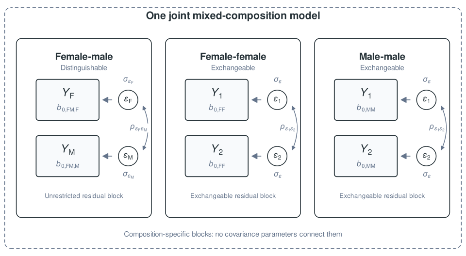
Diagram of one joint mixed-composition model containing three separate blocks. The female-male block has distinct female and male intercepts, separate residual variances, and their covariance. Female-female and male-male blocks each have one shared intercept, equal member residual variances, and a covariance. No covariance parameters connect the three composition blocks.

Structure of the cross-sectional mixed-composition APIM (Intercept only example). Female-male dyads have distinguishable member intercepts and an unrestricted residual covariance block. Each same-gender composition has a pooled intercept and an exchangeable residual covariance block. The three blocks are estimated jointly but are not connected by covariance parameters.

The model can then be specified as follows (example for an intercept-only model):


mixed_cross_gaussian_model <- glmmTMB::glmmTMB(
  satisfaction ~ 0 +

    ##### INTERCEPTS ######
    # fixed intercepts for individuals from distinguishable female-male couples
    .i_is_female_x_male_female + .i_is_female_x_male_male +

    # fixed pooled intercept for female-female couples
    .i_is_female_x_female +

    # fixed pooled intercept for male-male couples
    .i_is_male_x_male +

    ##### RESIDUAL STRUCTURE ######
    # distinguishable female-male residual covariance
    us(0 + .i_is_female_x_male_female + .i_is_female_x_male_male | coupleID) +

    # exchangeable female-female residual covariance via sum-diff
    us(0 + .i_is_female_x_female | coupleID) +
    us(0 + .i_diff_female_x_female_arbitrary | coupleID) +

    # exchangeable male-male residual covariance via sum-diff
    us(0 + .i_is_male_x_male | coupleID) +
    us(0 + .i_diff_male_x_male_arbitrary | coupleID)

  , dispformula = ~ 0
  , family = gaussian()
  , data = mixed_cross_data
)

summary(mixed_cross_gaussian_model)
#>  Family: gaussian  ( identity )
#> Formula:          
#> satisfaction ~ 0 + .i_is_female_x_male_female + .i_is_female_x_male_male +  
#>     .i_is_female_x_female + .i_is_male_x_male + us(0 + .i_is_female_x_male_female +  
#>     .i_is_female_x_male_male | coupleID) + us(0 + .i_is_female_x_female |  
#>     coupleID) + us(0 + .i_diff_female_x_female_arbitrary | coupleID) +  
#>     us(0 + .i_is_male_x_male | coupleID) + us(0 + .i_diff_male_x_male_arbitrary |  
#>     coupleID)
#> Dispersion:                    ~0
#> Data: mixed_cross_data
#> 
#>       AIC       BIC    logLik -2*log(L)  df.resid 
#>    2009.9    2059.0    -994.0    1987.9       629 
#> 
#> Random effects:
#> 
#> Conditional model:
#>  Groups     Name                              Variance Std.Dev. Corr  
#>  coupleID   .i_is_female_x_male_female        1.1999   1.0954         
#>             .i_is_female_x_male_male          1.9437   1.3942   -0.30 
#>  coupleID.1 .i_is_female_x_female             0.6682   0.8175         
#>  coupleID.2 .i_diff_female_x_female_arbitrary 0.3217   0.5672         
#>  coupleID.3 .i_is_male_x_male                 0.6274   0.7921         
#>  coupleID.4 .i_diff_male_x_male_arbitrary     1.0457   1.0226         
#> Number of obs: 640, groups:  coupleID, 320
#> 
#> Conditional model:
#>                            Estimate Std. Error z value Pr(>|z|)    
#> .i_is_female_x_male_female  5.50000    0.10000   55.00   <2e-16 ***
#> .i_is_female_x_male_male    4.50000    0.12727   35.36   <2e-16 ***
#> .i_is_female_x_female       5.80000    0.08175   70.95   <2e-16 ***
#> .i_is_male_x_male           4.20000    0.07921   53.02   <2e-16 ***
#> ---
#> Signif. codes:  0 '***' 0.001 '**' 0.01 '*' 0.05 '.' 0.1 ' ' 1

The same composition-specific blocks can be labelled directly from the fitted model. For the exchangeable blocks, the common member residual standard deviation and correlation are back-transformed from their fitted sum-and- difference components.

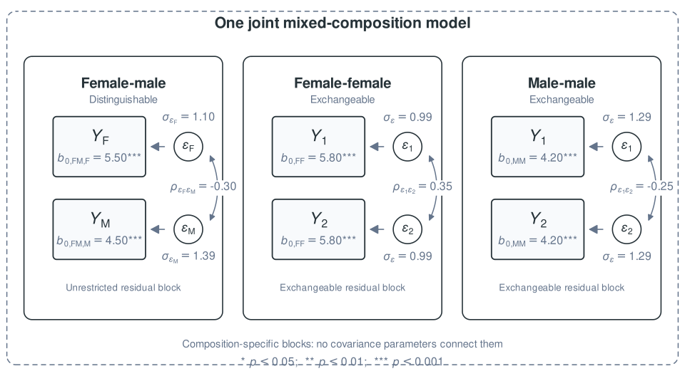
Fitted mixed-composition APIM. Female-male intercepts 5.50 and 4.50, residual SDs 1.10 and 1.39, and residual correlation -0.30. Female-female intercept 5.80, residual SD 0.99, and correlation 0.35. Male-male intercept 4.20, residual SD 1.29, and correlation -0.25.

Fitted intercept-only mixed-composition APIM. Intercepts and composition-specific residual parameters are extracted from the fitted joint model; the two exchangeable blocks are shown on the member scale.

The four fixed-effect indicators are mutually exclusive. With $I$ denoting the generated .i_is_{composition_role} indicator and $b_0$ a fixed intercept, the fixed part of the full model can be written as:

$\mu_{ij}^{\mathrm{fixed}} = b_{0,\mathrm{FM,F}} I_{\mathrm{FM,F},ij} + b_{0,\mathrm{FM,M}} I_{\mathrm{FM,M},ij} + b_{0,\mathrm{FF}} I_{\mathrm{FF},ij} + b_{0,\mathrm{MM}} I_{\mathrm{MM},ij}.$

In FM,F, the first part identifies the female-male composition and the final F identifies the female outcome member. The same composition-first convention is used throughout this vignette.

The active indicator for each person is shown below:

Row	$I_{\mathrm{FM,F}}$	$I_{\mathrm{FM,M}}$	$I_{\mathrm{FF}}$	$I_{\mathrm{MM}}$	Fixed intercept
Female in a female-male dyad	1	0	0	0	$b_{0,\mathrm{FM,F}}$
Male in a female-male dyad	0	1	0	0	$b_{0,\mathrm{FM,M}}$
Member of a female-female dyad	0	0	1	0	$b_{0,\mathrm{FF}}$
Member of a male-male dyad	0	0	0	1	$b_{0,\mathrm{MM}}$

Therefore, for a member of a male-male dyad, for example, the fixed part reduces to just $b_{0,\mathrm{MM}}$ via:

$0 \cdot b_{0,\mathrm{FM,F}} + 0 \cdot b_{0,\mathrm{FM,M}} + 0 \cdot b_{0,\mathrm{FF}} + 1 \cdot b_{0,\mathrm{MM}} = b_{0,\mathrm{MM}}.$

The random-effects terms reduce in the same way because their indicator columns are also 0 outside the relevant composition. The model combines an unrestricted distinguishable covariance block for female-male dyads with a separate equal-variance covariance block for each exchangeable composition. The main APIM vignette introduces the distinguishable and exchangeable structures.

The random-effects terms form composition-specific blocks, so no covariance parameters are estimated across compositions. Such parameters would not be identified because each dyad belongs to only one composition.

This illustration only covered the fixed-intercept model. The ILD example below shows how composition-specific slopes can be added.

Single versus separate mixed-composition fits

The mixed-composition models described in this vignette fit all dyad compositions in one model call. This is useful when the goal is to compare effects across compositions, test equality constraints, or make those comparisons within one joint fitted model.

marginaleffects::hypotheses() allows for testing linear combinations of glmmTMB fixed effects. In these equations, conditional_ identifies coefficients from the conditional model. A positive estimate means that the estimate on the left side is higher than the estimate on the right side.

# Test whether male-male and female-female pooled intercepts are different
marginaleffects::hypotheses(
  mixed_cross_gaussian_model,
  hypothesis = "conditional_.i_is_male_x_male = conditional_.i_is_female_x_female",
  re.form = NA
)

# Test whether the average female-male intercept is different from the pooled
# male-male intercept
marginaleffects::hypotheses(
  mixed_cross_gaussian_model,
  hypothesis = "(conditional_.i_is_female_x_male_female + conditional_.i_is_female_x_male_male) / 2 = conditional_.i_is_male_x_male",
  re.form = NA
)

# Test whether the male intercept from a female-male couple is different from
# the pooled male intercept from a male-male couple
marginaleffects::hypotheses(
  mixed_cross_gaussian_model,
  hypothesis = "conditional_.i_is_female_x_male_male = conditional_.i_is_male_x_male",
  re.form = NA
)

Since we only want to compare fixed-effects here, we set re.form = NA.

It is important to note that such a fixed-effect formula with all compositions in one model call does not create partial pooling across dyad compositions. Estimates for female-female, for instance, are not automatically shrunk toward estimates from the other dyad types. In this model, almost every parameter is composition-specific. This means that the likelihood largely factorizes by composition. Therefore, separate composition-specific fits would largely recover the same parameters.

The main advantage of estimating everything in a single model is that formal parameter comparisons can be made within one fitted model, and that models with different versions of pooling can be compared. For example, it can be tested whether pooling male-male and female-female couples as same-sex substantially worsens model fit, considering both the fixed effects and random-effects structure. Such model comparisons require the restricted and unrestricted models to use the same observations and require the restricted model to be nested within the unrestricted model.

If partial pooling is desired, for instance with few dyads for one particular type, a different model specification would be required, such as a common effect plus composition deviations.

Model comparison with a restricted model

The regular APIM vignette introduces compare_interdep_models() by comparing a distinguishable APIM with its exchangeable restriction. Here, we use the same approach for a mixed-composition constraint. We treat female-male dyads as exchangeable and pool them with male-male dyads, while modeling female-female dyads separately. In an applied analysis, these constraints would require a theoretical or empirical justification.

mixed_cross_data_constrained <- prepare_interdep_data(
  example_dyadic_crosssectional_mixed,
  group = coupleID,
  member = personID,
  role = gender,
  set_exchangeable_compositions = "male-female",
  pool_compositions = list(
    "non_female_x_female" = c("male-male", "female-male")
  ),
  seed = 123
)

mixed_cross_gaussian_model_constrained <- glmmTMB::glmmTMB(
  satisfaction ~ 0 +
    .i_is_female_x_female +
    .i_is_non_female_x_female +

    # exchangeable female-female residual covariance via sum-diff
    us(0 + .i_is_female_x_female | coupleID) +
    us(0 + .i_diff_female_x_female_arbitrary | coupleID) +

    # pooled female-male and male-male residual covariance via sum-diff
    us(0 + .i_is_non_female_x_female | coupleID) +
    us(0 + .i_diff_non_female_x_female_arbitrary | coupleID)

  , dispformula = ~ 0
  , family = gaussian()
  , data = mixed_cross_data_constrained
)

compare_interdep_models(
  restricted = mixed_cross_gaussian_model_constrained,
  full = mixed_cross_gaussian_model
)
#> Likelihood-ratio test for nested models fitted to equivalent interdep data
#> Mathematical nesting is assumed and cannot be verified from the data alone.
#> 
#>                                        Df    AIC    BIC   logLik deviance
#> mixed_cross_gaussian_model_constrained  6 2087.8 2114.6 -1037.90   2075.8
#> mixed_cross_gaussian_model             11 2010.0 2059.0  -993.97   1988.0
#>                                         Chisq Chi Df Pr(>Chisq)    
#> mixed_cross_gaussian_model_constrained                             
#> mixed_cross_gaussian_model             87.856      5  < 2.2e-16 ***
#> ---
#> Signif. codes:  0 '***' 0.001 '**' 0.01 '*' 0.05 '.' 0.1 ' ' 1
#> 
#> Under the assumed nesting and chi-squared reference distribution, the test provides evidence that `mixed_cross_gaussian_model_constrained` fits the data worse than `mixed_cross_gaussian_model` (likelihood-ratio test: χ²(5) = 87.86, p < .001).

Here, the constrained model fits substantially worse than the full model. Note that the test evaluates all imposed constraints jointly, including the pooled fixed effects and residual covariance structure. It does not show which restriction accounts for the difference.

Mixed-composition intensive longitudinal (ILD) Gaussian model

example_dyadic_ILD_mixed contains the same three dyad compositions as the mixed-composition cross-sectional example, but each dyad contributes repeated paired observations over diaryday.

To keep the example lighter, we pool female-female and male-male dyads into one same-sex composition. This is a simplifying modeling assumption and does not reflect all differences used to simulate these example data. In an applied analysis, pooling should be theoretically justified or evaluated by comparing pooled and unpooled models fitted to the same observations.

Aside from the pooling, we prepare the data in the same way, now adding time and a predictor:

mixed_ild_data <- prepare_interdep_data(
  example_dyadic_ILD_mixed,
  group = coupleID,
  member = personID,
  role = gender,
  pool_compositions = list(
    "same-sex" = c("male-male", "female-female")
  ),
  time = diaryday,
  predictors = provided_support,
  seed = 123
)

print(mixed_ild_data)
#> # interdep data
#> # Rows: 5600 | Dyads: 200 | Intensive longitudinal: yes
#> # Structure: group = coupleID, member = personID, role = gender, time =
#> # diaryday
#> #
#> # Dyad compositions:
#> # female_x_male          distinguishable  80 dyads
#> # same-sex (pooled)      exchangeable    120 dyads
#> #   female_x_female
#> #   male_x_male
#> #
#> # Added columns:
#> #   .i_composition         inferred dyad composition
#> #   .i_composition_role    composition-specific member role
#> #   .i_is_{comp-role}      composition-role indicator columns
#> #   .i_diff_{comp}         composition-specific sum-diff contrasts with
#> #                          arbitrary direction; 0 for distinguishable dyads or
#> #                          other exchangeable compositions
#> #   .i_{pred}_cwp          within-person predictor: momentary deviations from
#> #                          each person's usual level
#> #   .i_{pred}_cbp          between-person predictor: stable differences from
#> #                          the average person's usual level
#> #   .i_{pred}_actor        APIM actor predictor: actor's original predictor
#> #                          values
#> #   .i_{pred}_partner      APIM partner predictor: partner's original predictor
#> #                          values
#> #   .i_{pred}_cwp_actor    APIM within-person actor predictor: actor's
#> #                          momentary deviations from their usual level
#> #   .i_{pred}_cwp_partner  APIM within-person partner predictor: partner's
#> #                          momentary deviations from their usual level
#> #   .i_{pred}_cbp_actor    APIM between-person actor predictor: actor's stable
#> #                          difference from the average person's usual level
#> #   .i_{pred}_cbp_partner  APIM between-person partner predictor: partner's
#> #                          stable difference from the average person's usual
#> #                          level
#> #
#> # A tibble: 5,600 × 20
#>    personID coupleID diaryday gender closeness provided_support .i_composition
#>       <int>    <int>    <int> <fct>      <dbl>            <dbl> <fct>         
#>  1        1        1        0 female      3.79             4.85 female_x_male 
#>  2        1        1        1 female      2.89             4.13 female_x_male 
#>  3        1        1        2 female      4.20             4.62 female_x_male 
#>  4        1        1        3 female      5.79             5.09 female_x_male 
#>  5        1        1        4 female      3.97             4.92 female_x_male 
#>  6        1        1        5 female      3.53             4.51 female_x_male 
#>  7        1        1        6 female      4.38             5.09 female_x_male 
#>  8        1        1        7 female      3.51             4.92 female_x_male 
#>  9        1        1        8 female      4.45             4.11 female_x_male 
#> 10        1        1        9 female      3.17             4.01 female_x_male 
#> # ℹ 5,590 more rows
#> # ℹ 13 more variables: .i_composition_role <fct>,
#> #   .i_is_female_x_male_female <dbl>, .i_is_female_x_male_male <dbl>,
#> #   .i_is_same_sex <dbl>, .i_diff_same_sex_arbitrary <dbl>,
#> #   .i_provided_support_cwp <dbl>, .i_provided_support_cbp <dbl>,
#> #   .i_provided_support_actor <dbl>, .i_provided_support_partner <dbl>,
#> #   .i_provided_support_cwp_actor <dbl>, …

Note that observed person means used to construct the between-person (cbp) predictors can be unreliable when each member contributes few occasions, which can bias between-person estimates (Gottfredson 2019).

This mixed-composition ILD model includes composition-specific fixed intercepts, time slopes, and within-person and between-person actor and partner effects. It omits random slopes, as they would add several variances and covariances to an already large model.

This model is complex and may produce optimizer convergence warnings, especially when the random-effects structure is too complex for the available data or some components are close to zero (del Rosario and West 2025). When near-zero covariance components make a frequentist fit unstable, regularizing priors in a Bayesian model can sometimes help, but they do not replace careful model checks (del Rosario and West 2025). A Bayesian implementation of this mixed-composition model is beyond the scope of this vignette. For these example data, we use the BFGS optimizer with a higher iteration limit.


mixed_ild_gaussian_model <- glmmTMB::glmmTMB(
  closeness ~ 0 +

    # Composition-specific intercepts
    .i_is_female_x_male_female + .i_is_female_x_male_male +

    .i_is_same_sex +

    # Composition-specific time trends
    .i_is_female_x_male_female:diaryday +
    .i_is_female_x_male_male:diaryday +

    .i_is_same_sex:diaryday +

    # Composition-specific within-person actor effects
    .i_is_female_x_male_female:.i_provided_support_cwp_actor +
    .i_is_female_x_male_male:.i_provided_support_cwp_actor +

    .i_is_same_sex:.i_provided_support_cwp_actor +

    # Composition-specific within-person partner effects
    .i_is_female_x_male_female:.i_provided_support_cwp_partner +
    .i_is_female_x_male_male:.i_provided_support_cwp_partner +

    .i_is_same_sex:.i_provided_support_cwp_partner +

    # Composition-specific between-person actor effects
    .i_is_female_x_male_female:.i_provided_support_cbp_actor +
    .i_is_female_x_male_male:.i_provided_support_cbp_actor +

    .i_is_same_sex:.i_provided_support_cbp_actor +

    # Composition-specific between-person partner effects
    .i_is_female_x_male_female:.i_provided_support_cbp_partner +
    .i_is_female_x_male_male:.i_provided_support_cbp_partner +

    .i_is_same_sex:.i_provided_support_cbp_partner +

    # stable dyad-level covariance
    us(0 + .i_is_female_x_male_female + .i_is_female_x_male_male | coupleID) +

    us(0 + .i_is_same_sex | coupleID) +
    us(0 + .i_diff_same_sex_arbitrary | coupleID) +

    # same-day covariance
    us(0 + .i_is_female_x_male_female + .i_is_female_x_male_male | coupleID:diaryday) +

    us(0 + .i_is_same_sex | coupleID:diaryday) +
    us(0 + .i_diff_same_sex_arbitrary | coupleID:diaryday)

  , dispformula = ~ 0
  , family = gaussian()
  , data = mixed_ild_data
  , control = glmmTMB::glmmTMBControl(
      optimizer = stats::optim,
      optArgs = list(method = "BFGS"),
      optCtrl = list(maxit = 10000)
    )
)

summary(mixed_ild_gaussian_model)

This example omits random slopes, as they would add further complexity. To extend the model with random slopes, the following blocks would replace the stable dyad-level covariance terms in the model above:

# distinguishable female-male random intercepts and slopes
us(
  0 +
    .i_is_female_x_male_female +
    .i_is_female_x_male_male +
    .i_is_female_x_male_female:.i_provided_support_cwp_actor +
    .i_is_female_x_male_male:.i_provided_support_cwp_actor +
    .i_is_female_x_male_female:.i_provided_support_cwp_partner +
    .i_is_female_x_male_male:.i_provided_support_cwp_partner |
    coupleID
) +

# exchangeable same-sex shared block
us(
  0 +
    .i_is_same_sex +
    .i_is_same_sex:.i_provided_support_cwp_actor +
    .i_is_same_sex:.i_provided_support_cwp_partner |
    coupleID
) +

# exchangeable same-sex difference block
us(
  0 +
    .i_diff_same_sex_arbitrary +
    .i_diff_same_sex_arbitrary:.i_provided_support_cwp_actor +
    .i_diff_same_sex_arbitrary:.i_provided_support_cwp_partner |
    coupleID
)

This extension estimates a very large covariance structure and may not be supported by many datasets. Regularizing priors in a Bayesian framework may help with estimation, but they do not necessarily make an unsupported random-effects structure appropriate.

Takeaway

Mixed dyad compositions do not always require separate models. interdep creates the necessary columns to fit a joint model and apply various pooling and exchangeability constraints.

It is often useful to begin with separate composition-specific models or simpler covariance structures. Combine them when an equality constraint or a comparison of effects across compositions is part of the research question, and add further random effects only when the data support the additional complexity.

Return to the Actor-Partner Interdependence Model vignette, see the Dyad-Individual Model vignette or the Dyadic Score Model vignette for alternative parameterizations, or return to the Overview.

References

Bolger, Niall, Jean-Philippe Laurenceau, and Ana DiGiovanni. 2025. “Unified Analysis Model for Indistinguishable and Distinguishable Dyads.” Innovations in Interpersonal Relationships and Health Research: Advancing the Integration of Interdisciplinary Approaches to Dyadic Behavior Change. https://doi.org/10.17605/OSF.IO/WYDCJ.

Gottfredson, Nisha C. 2019. “A Straightforward Approach for Coping with Unreliability of Person Means When Parsing Within-Person and Between-Person Effects in Longitudinal Studies.” Addictive Behaviors 94: 156–61. https://doi.org/10.1016/j.addbeh.2018.09.031.