Actor-Partner Interdependence Model (APIM)

Pascal Küng

library(interdep)

This vignette focuses on the cross-sectional and intensive longitudinal Actor-Partner Interdependence model for distinguishable and exchangeable dyads.

For the broader package workflow and an overview of the available model-specific vignettes, including the Mixed-Composition APIM, Dyad-Individual Model, and Dyadic Score Model, see the Overview.

This vignette is under construction and preliminary. Please check back soon!

The cross sectional Gaussian distinguishable APIM

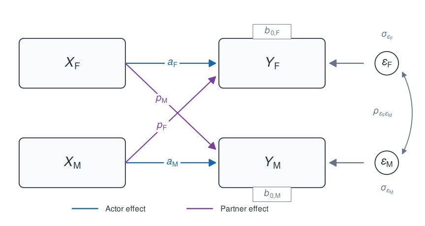
Conceptual cross-sectional APIM for distinguishable female-male dyads. Intercepts, actor effects, and partner effects can differ by the role of the outcome member, and the two outcome residuals covary within dyads.

Here, $b_{\mathrm{actor},\mathrm{female}}$ and $b_{\mathrm{actor},\mathrm{male}}$ are the actor effects on the female and male outcomes, whereas $b_{\mathrm{partner},\mathrm{female}}$ and $b_{\mathrm{partner},\mathrm{male}}$ are the corresponding partner effects. The diagram abbreviates these paths as $a_{\mathrm{F}}$, $a_{\mathrm{M}}$, $p_{\mathrm{F}}$, and $p_{\mathrm{M}}$, with the subscript identifying the outcome member. In the text and equations, fixed coefficients use $b$ and write out actor and partner explicitly. The corresponding intercepts are $b_{0,\mathrm{female}}$ and $b_{0,\mathrm{male}}$. All four paths can differ in a distinguishable APIM.

The conceptual diagram places both members in one SEM-style path model. The same model is fitted in long format with one outcome row per member. In the individual-level representation below, the female predictor is the actor predictor for the female outcome and the partner predictor for the male outcome; the male predictor changes roles in the same way. The coefficient subscript identifies the outcome member.

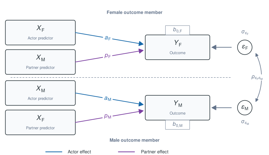
Individual-level representation of the distinguishable cross-sectional APIM used for the long-format multilevel model. For the female outcome, the female predictor is the actor predictor and the male predictor is the partner predictor; these roles reverse for the male outcome. Intercepts, actor coefficients, and partner coefficients may differ by outcome role, and the two member residuals may have different variances and covary.

We first prepare the example data with prepare_interdep_data():

apim_distinguishable_data <- prepare_interdep_data(
  data = example_dyadic_crosssectional,
  group = coupleID,
  member = personID,
  role = gender,
  predictors = communication,
  model_type = "apim"
)

The generated .i_* columns can be used directly in the model formula. Here is a simple example:

apim_distinguishable_model <- glmmTMB::glmmTMB(
  satisfaction ~

    # Gender-specific intercepts
    0 +
    .i_is_female_x_male_female +
    .i_is_female_x_male_male +

    # Gender-specific actor effects
    .i_is_female_x_male_female:.i_communication_actor +
    .i_is_female_x_male_male:.i_communication_actor +

    # Gender-specific partner effects
    .i_is_female_x_male_female:.i_communication_partner +
    .i_is_female_x_male_male:.i_communication_partner +

    # Dyad-level unstructured random effects represent the two partner
    # residual variances and their covariance when dispformula = ~ 0.
    # This is glmmTMB-specific syntax! lme4 and brms use different syntax.
    us(0 +
         .i_is_female_x_male_female +
         .i_is_female_x_male_male
       | coupleID)

  , dispformula = ~ 0
  , family = gaussian()
  , data = apim_distinguishable_data
)

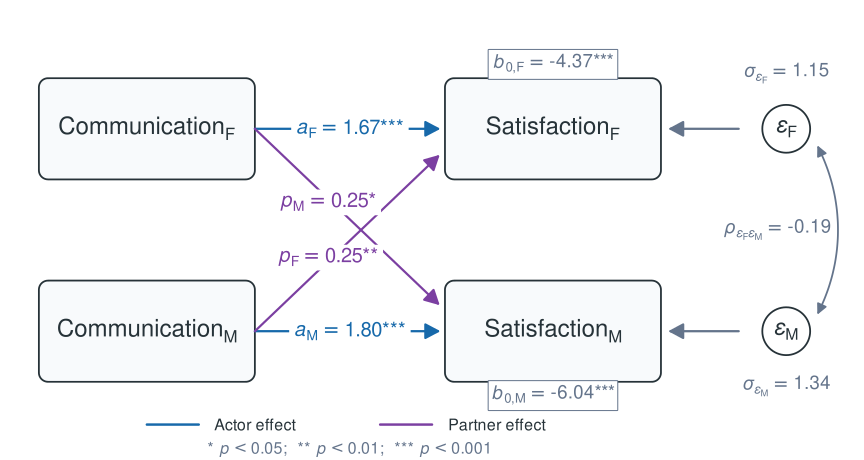
Fitted cross-sectional distinguishable APIM for the example data. Fixed effects, residual standard deviations, and the residual correlation are extracted from the fitted model.

Residual random-effects structure

For a distinguishable female-male dyad, the two members can have different residual variances. Their residual covariance matrix is

$$\boldsymbol{\Sigma}_{\mathrm{FM}} = \begin{pmatrix} \sigma_{\mathrm{FM,F}}^2 & c_{\mathrm{FM}} \\ c_{\mathrm{FM}} & \sigma_{\mathrm{FM,M}}^2 \end{pmatrix}.$$

Rows and columns are ordered female, male.

With one outcome row per member, this structure is estimated with an unstructured random-effects block such as us(0 + .i_is_female_x_male_female + .i_is_female_x_male_male | coupleID) and dispformula = ~ 0. The two indicator columns select the female and male rows, respectively. The us() block estimates both variances and their covariance.

Interpretation

The cross-sectional Gaussian exchangeable APIM

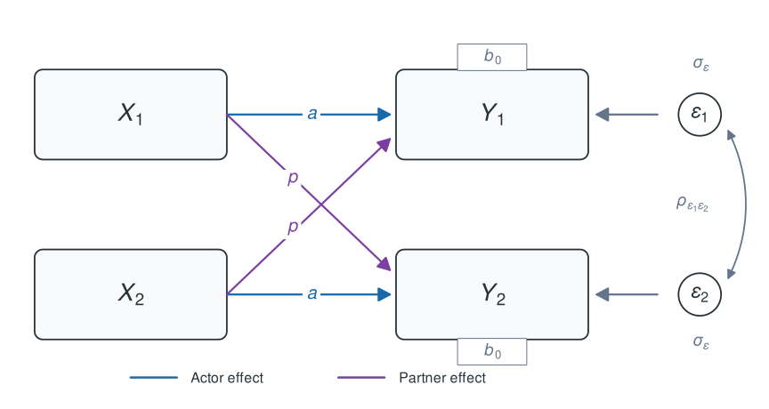
Conceptual cross-sectional APIM for exchangeable dyads. The two members share one intercept, one actor effect, and one partner effect; their outcome residuals have equal variances and covary within dyads.

Because the member labels are arbitrary, swapping members 1 and 2 does not change the model. The two actor paths therefore share the coefficient $b_{\mathrm{actor}}$, and the two partner paths share $b_{\mathrm{partner}}$. The members also share the intercept $b_0$. The two residual variances are constrained to be equal, while their covariance is estimated. The diagram abbreviates the shared actor and partner effects as $a$ and $p$.

The individual-level representation makes the long-format model explicit. For each outcome row, that member’s own predictor is the actor predictor and the other member’s predictor is the partner predictor. Swapping the arbitrary member labels swaps the two panels but does not change either coefficient.

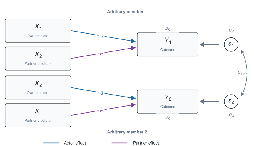
Individual-level representation of the exchangeable cross-sectional APIM used for the long-format multilevel model. Both members share the same intercept. Each member’s own predictor has the shared actor effect, and the other member’s predictor has the shared partner effect. The two residual variances are equal and the residuals may covary.

Assumptions

Residual random-effects structure and back-transformation

For an exchangeable dyad, interdep generates an arbitrary member-difference column, named .i_diff_*, that is +1 for one member and -1 for the other. The exchangeable residual structure is represented by two separate random-effects terms: a shared dyad random intercept and a random coefficient for this difference column (del Rosario and West 2025). If their random effects are denoted by $u_{\mathrm{mean},j}$ and $u_{\mathrm{diff},j}$, the two members receive

$$r_{1j} = u_{\mathrm{mean},j} + u_{\mathrm{diff},j}, \qquad r_{2j} = u_{\mathrm{mean},j} - u_{\mathrm{diff},j}.$$

Because the shared and difference effects are fitted in separate random-effects terms, they are uncorrelated. Writing their variances as $\sigma_{\mathrm{mean}}^2$ and $\sigma_{\mathrm{diff}}^2$ gives

$$\begin{pmatrix} u_{\mathrm{mean},j} \\ u_{\mathrm{diff},j} \end{pmatrix} \sim \mathcal{N} \left[ \begin{pmatrix} 0 \\ 0 \end{pmatrix}, \begin{pmatrix} \sigma_{\mathrm{mean}}^2 & 0 \\ 0 & \sigma_{\mathrm{diff}}^2 \end{pmatrix} \right].$$

The implied member-level residual covariance matrix is therefore

$$\boldsymbol{\Sigma}_{\mathrm{exch}} = \begin{pmatrix} \sigma_{\mathrm{mean}}^2 + \sigma_{\mathrm{diff}}^2 & \sigma_{\mathrm{mean}}^2 - \sigma_{\mathrm{diff}}^2 \\ \sigma_{\mathrm{mean}}^2 - \sigma_{\mathrm{diff}}^2 & \sigma_{\mathrm{mean}}^2 + \sigma_{\mathrm{diff}}^2 \end{pmatrix}.$$

Thus, both members have the same residual variance $v = \sigma_{\mathrm{mean}}^2 + \sigma_{\mathrm{diff}}^2$, their covariance is $c = \sigma_{\mathrm{mean}}^2 - \sigma_{\mathrm{diff}}^2$, and their residual correlation is $c/v$. Conversely, the shared and difference variances can be recovered from a member-level variance and covariance as

$$\sigma_{\mathrm{mean}}^2 = \frac{v + c}{2}, \qquad \sigma_{\mathrm{diff}}^2 = \frac{v - c}{2}.$$

For example, a random-intercept variance of 1.2 and a difference variance of 0.3 imply a member variance of 1.5 and a covariance between partners of 0.9.

Reversing the arbitrary +1/-1 assignment changes the sign of $u_{\mathrm{diff},j}$ but not its variance or the implied member-level covariance matrix. In longitudinal models, the same transformation applies separately to stable dyad-level and same-occasion dyad-level covariance blocks.

Extension to exchangeable random slopes

The same shared/difference back-transformation applies to random slopes (del Rosario and West 2025). For example, let $u_{\mathrm{actor},j}$ denote the shared actor random slope for dyad $j$ and $\widetilde{u}_{\mathrm{actor},j}$ the corresponding .i_diff_* random slope. The tilde marks random coefficients from the member-difference block. The actor slopes for the members assigned +1 and -1 are

$$u_{\mathrm{actor},1j} = u_{\mathrm{actor},j} + \widetilde{u}_{\mathrm{actor},j}, \qquad u_{\mathrm{actor},2j} = u_{\mathrm{actor},j} - \widetilde{u}_{\mathrm{actor},j}.$$

Because the shared and .i_diff_* blocks are fitted as separate random-effects terms, they are independent. Therefore,

$$\operatorname{Var}(u_{\mathrm{actor},1j}) = \operatorname{Var}(u_{\mathrm{actor},2j}) = \operatorname{Var}(u_{\mathrm{actor},j}) + \operatorname{Var}(\widetilde{u}_{\mathrm{actor},j}),$$

and

$$\operatorname{Cov}(u_{\mathrm{actor},1j}, u_{\mathrm{actor},2j}) = \operatorname{Var}(u_{\mathrm{actor},j}) - \operatorname{Var}(\widetilde{u}_{\mathrm{actor},j}).$$

The same calculation applies to the partner slopes and random intercepts. Any covariances among the random intercept, actor slope, and partner slope can be back-transformed in the same way.

Interpretation

Testing distinguishability

Distinguishability can be evaluated by comparing a full model in which the two roles may differ with a restricted exchangeable model. This comparison tests the imposed equality constraints jointly. Here, they concern the fixed intercepts, actor effects, partner effects, and residual variances.

The two parameterizations require different generated columns. The full distinguishable model was fitted above, so we now prepare the same original observations as exchangeable:

apim_exchangeable_data <- prepare_interdep_data(
  example_dyadic_crosssectional,
  group = coupleID,
  member = personID,
  role = gender,
  predictors = communication,
  set_exchangeable_compositions = "female-male"
)

The exchangeable model constrains the corresponding fixed effects and residual variances to be equal across members:

apim_exchangeable_model <- glmmTMB::glmmTMB(
  satisfaction ~ 0 +
    .i_is_female_x_male +
    .i_communication_actor +
    .i_communication_partner +
    us(0 + .i_is_female_x_male | coupleID) +
    us(0 + .i_diff_female_x_male_arbitrary | coupleID),
  dispformula = ~ 0,
  family = gaussian(),
  data = apim_exchangeable_data
)

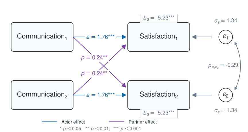
Fitted cross-sectional exchangeable APIM for the example data. The common member residual standard deviation and residual correlation are back-transformed from the fitted mean and difference components.

compare_interdep_models() verifies that both models use equivalent original observations before performing the likelihood-ratio test:

compare_interdep_models(
  restricted = apim_exchangeable_model,
  full = apim_distinguishable_model
)
#> Likelihood-ratio test for nested models fitted to equivalent interdep data
#> Mathematical nesting is assumed and cannot be verified from the data alone.
#> 
#>                            Df    AIC    BIC  logLik deviance  Chisq Chi Df
#> apim_exchangeable_model     5 603.98 619.84 -296.99   593.98              
#> apim_distinguishable_model  9 589.49 618.03 -285.75   571.49 22.492      4
#>                            Pr(>Chisq)    
#> apim_exchangeable_model                  
#> apim_distinguishable_model  0.0001599 ***
#> ---
#> Signif. codes:  0 '***' 0.001 '**' 0.01 '*' 0.05 '.' 0.1 ' ' 1
#> 
#> Under the assumed nesting and chi-squared reference distribution, the test provides evidence that `apim_exchangeable_model` fits the data worse than `apim_distinguishable_model` (likelihood-ratio test: χ²(4) = 22.49, p < .001).

The test provides evidence against all restrictions jointly, but it does not show which parameter differs. The helper also cannot determine whether the models are mathematically nested; that remains a modeling requirement. The usual chi-squared reference distribution may be unreliable when a tested variance parameter lies on its boundary.

Intensive longitudinal APIMs

Concurrent ILD Gaussian APIM for distinguishable dyads

Observed person means used to construct the between-person (cbp) predictors can be unreliable when each member contributes few occasions, which can bias between-person estimates (Gottfredson 2019).

Example model specification:

ild_distinguishable_model <- glmmTMB(
  closeness ~ 0 + 
    
    .i_is_female_x_male_female + 
    .i_is_female_x_male_male + 
    
    # Gender specific time trends
    .i_is_female_x_male_female:diaryday + 
    .i_is_female_x_male_male:diaryday +
    
    # Gender-specific within-person actor effects
    .i_is_female_x_male_female:.i_provided_support_cwp_actor +
    .i_is_female_x_male_male:.i_provided_support_cwp_actor +

    # Gender-specific within-person partner effects
    .i_is_female_x_male_female:.i_provided_support_cwp_partner +
    .i_is_female_x_male_male:.i_provided_support_cwp_partner +
    
    # Gender-specific between-person actor effects
    .i_is_female_x_male_female:.i_provided_support_cbp_actor +
    .i_is_female_x_male_male:.i_provided_support_cbp_actor +

    # Gender-specific between-person partner effects
    .i_is_female_x_male_female:.i_provided_support_cbp_partner +
    .i_is_female_x_male_male:.i_provided_support_cbp_partner +
    
    # random effects for stable non-independence (means)
    us(0 + 
         .i_is_female_x_male_female + 
         .i_is_female_x_male_male 
       | coupleID)  +

    # Same-day residual covariance
    us(0 + 
         .i_is_female_x_male_female + 
         .i_is_female_x_male_male 
       | coupleID:diaryday) 

  , dispformula = ~ 0  
  , family = gaussian()
  , data = ild_distinguishable_data
)

summary(ild_distinguishable_model)

Concurrent ILD Gaussian APIM for exchangeable dyads

Following del Rosario and West, the stable dyad covariance can be represented using sum-and-difference random effects (del Rosario and West 2025). In longitudinal Gaussian APIMs fitted with glmmTMB, the same parameterization can be extended to the dyad-occasion level to represent same-occasion residual dependence.

Current limitations of dyadic ILD designs in R

Concurrent dyadic ILD models can adjust for a time trend and account for stable dyadic dependence and same-occasion partner dependence. They do not model residual serial dependence, however, and therefore estimate concurrent associations under the assumption that residuals from different days are independent.

If the goal is to retain these concurrent APIM associations while accounting for serial dependence, the closest extension is a dyadic residual dynamic structural equation model (RDSEM). It keeps the concurrent regression separate from a VAR model for its residuals (Asparouhov and Muthén 2020; McNeish and Hamaker 2020). This residual-VAR structure is not directly available through the glmmTMB interface used here, and open-source support for dyadic dynamic models remains very limited (del Rosario and West 2025). Within open-source R, such a model generally requires custom TMB or Stan code.

Dynamic models

A practical alternative is a model with lagged outcomes, especially when carryover or temporal dynamics are part of the research question (Gistelinck and Loeys 2020). In such a model, the interpretation changes. All APIM predictor effects then describe associations conditional on the members’ prior outcomes.

By adding the outcome to predictors and selecting it with lag_predictors, prepare_interdep_data() returns lag-1 raw and within-person scores alongside the contemporaneous scores. Between-person scores are not lagged because they describe stable differences between members.

For this example, we obtain the lagged actor and partner outcome columns through the lag_predictors argument:

ild_apim_data_dynamic <- prepare_interdep_data(
  example_dyadic_ILD,
  group = coupleID,
  member = personID,
  time = diaryday,
  predictors = closeness,
  lag_predictors = closeness,
  model_type = "apim",
  seed = 123
)

This returns all necessary variables for either choice, including lag-1 raw and within-person closeness scores. Lags are matched at exactly diaryday - 1, so omitted diary days are not bridged.

A simple fixed-slope dyadic stability and influence model (del Rosario and West 2025):

stability_influence <- glmmTMB::glmmTMB(
  closeness ~ 1 +

    # Stability (actor effect across time)
    .i_closeness_actor_lag1 +

    # Influence (partner effect across time)
    .i_closeness_partner_lag1 +

    # Linear time trend
    diaryday +

    # Stable exchangeable dyad-level covariance
    us(1 | coupleID) +
    us(0 + .i_diff_assumed_exchangeable_arbitrary | coupleID) +

    # Same-day exchangeable dyad-level covariance
    us(1 | coupleID:diaryday) +
    us(0 + .i_diff_assumed_exchangeable_arbitrary | coupleID:diaryday)

  , dispformula = ~ 0
  , family = gaussian()
  , data = ild_apim_data_dynamic
)

summary(stability_influence)
#>  Family: gaussian  ( identity )
#> Formula:          
#> closeness ~ 1 + .i_closeness_actor_lag1 + .i_closeness_partner_lag1 +  
#>     diaryday + us(1 | coupleID) + us(0 + .i_diff_assumed_exchangeable_arbitrary |  
#>     coupleID) + us(1 | coupleID:diaryday) + us(0 + .i_diff_assumed_exchangeable_arbitrary |  
#>     coupleID:diaryday)
#> Dispersion:                 ~0
#> Data: ild_apim_data_dynamic
#> 
#>       AIC       BIC    logLik -2*log(L)  df.resid 
#>    2929.0    2968.0   -1456.5    2913.0       967 
#> 
#> Random effects:
#> 
#> Conditional model:
#>  Groups              Name                                   Variance Std.Dev.
#>  coupleID            (Intercept)                            0.9161   0.9571  
#>  coupleID.1          .i_diff_assumed_exchangeable_arbitrary 0.5742   0.7578  
#>  coupleID.diaryday   (Intercept)                            0.3925   0.6265  
#>  coupleID.diaryday.1 .i_diff_assumed_exchangeable_arbitrary 0.5234   0.7235  
#> Number of obs: 975, groups:  coupleID, 40; coupleID:diaryday, 497
#> 
#> Conditional model:
#>                            Estimate Std. Error z value Pr(>|z|)    
#> (Intercept)                4.213055   0.300180  14.035  < 2e-16 ***
#> .i_closeness_actor_lag1    0.143976   0.035326   4.076 4.59e-05 ***
#> .i_closeness_partner_lag1  0.028761   0.035386   0.813    0.416    
#> diaryday                  -0.005280   0.007643  -0.691    0.490    
#> ---
#> Signif. codes:  0 '***' 0.001 '**' 0.01 '*' 0.05 '.' 0.1 ' ' 1

This model can be extended with contemporaneous actor and partner predictor associations and other lagged predictors. Time-varying predictors should usually be separated into within-person and between-person components. Their contemporaneous coefficients are then conditional on both partners’ prior outcomes.

The model above uses raw lagged outcomes. The corresponding within-person-centered lagged terms are .i_closeness_cwp_actor_lag1 and .i_closeness_cwp_partner_lag1.

Whether to use a raw or within-person-centered lagged outcome depends on the research question and the data. Person-mean centering the outcome lag can bias the average carryover estimate downward (Hamaker and Grasman 2015). This downward bias is known as Nickell bias (Nickell 1981). A raw lag avoids this centering bias, but a standard random-intercept model can still be biased because it assumes that the lag is unrelated to stable member levels (Gistelinck et al. 2021).

Both problems matter most when there are few occasions. In one simple simulation, most approaches other than person-mean centering performed acceptably from about ten occasions, but this is not a universal cutoff (Gistelinck et al. 2021). For shorter panels, consider an LD-APIM, which lets the first outcomes relate to the members’ stable levels in a wide-format SEM (Gistelinck and Loeys 2020).

These manifest-lag models are not equivalent to Mplus DSEM, which uses latent person-mean centering by default and can estimate multivariate or residual dynamics jointly (McNeish and Hamaker 2020). For very short panels, however, default DSEM may still be biased or unstable, so the LD-APIM recommendation above may be preferable (Gistelinck et al. 2021).

These lagged-outcome issues are separate from the earlier concern about unreliable person means used to construct cbp predictors with few occasions.

---

From here, choose the model-specific vignette that matches the research question:

• Mixed-Composition APIM vignette for analyses combining distinguishable and exchangeable dyad compositions;
• Dyad-Individual Model vignette for the exchangeable DIM parameterization; or
• Dyadic Score Model vignette for the distinguishable DSM parameterization.

Or return to the Overview.

A vignette with non-Gaussian generalized APIM examples is planned.

References

Asparouhov, Tihomir, and Bengt Muthén. 2020. “Comparison of Models for the Analysis of Intensive Longitudinal Data.” Structural Equation Modeling: A Multidisciplinary Journal 27 (2): 275–97. https://doi.org/10.1080/10705511.2019.1626733.

Gistelinck, Fien, and Tom Loeys. 2020. “Multilevel Autoregressive Models for Longitudinal Dyadic Data.” TPM - Testing, Psychometrics, Methodology in Applied Psychology 27 (3): 433–52. https://doi.org/10.4473/TPM27.3.7.

Gistelinck, Fien, Tom Loeys, and Nele Flamant. 2021. “Multilevel Autoregressive Models When the Number of Time Points Is Small.” Structural Equation Modeling: A Multidisciplinary Journal 28 (1): 15–27. https://doi.org/10.1080/10705511.2020.1753517.

Gottfredson, Nisha C. 2019. “A Straightforward Approach for Coping with Unreliability of Person Means When Parsing Within-Person and Between-Person Effects in Longitudinal Studies.” Addictive Behaviors 94: 156–61. https://doi.org/10.1016/j.addbeh.2018.09.031.

Hamaker, Ellen L., and Raoul P. P. P. Grasman. 2015. “To Center or Not to Center? Investigating Inertia with a Multilevel Autoregressive Model.” Frontiers in Psychology 5: 1492. https://doi.org/10.3389/fpsyg.2014.01492.

McNeish, Daniel, and Ellen L. Hamaker. 2020. “A Primer on Two-Level Dynamic Structural Equation Models for Intensive Longitudinal Data in Mplus.” Psychological Methods 25 (5): 610–35. https://doi.org/10.1037/met0000250.

Nickell, Stephen. 1981. “Biases in Dynamic Models with Fixed Effects.” Econometrica 49 (6): 1417–26. https://doi.org/10.2307/1911408.

Rosario, Kareena S. del, and Tessa V. West. 2025. “A Practical Guide to Specifying Random Effects in Longitudinal Dyadic Multilevel Modeling.” Advances in Methods and Practices in Psychological Science 8 (3): 25152459251351286. https://doi.org/10.1177/25152459251351286.