Dyad-Individual Model

Pascal Küng

library(interdep)
has_glmmTMB <- requireNamespace("glmmTMB", quietly = TRUE)
dim_fitted_alt <- "Fitted DIM diagram unavailable."

This vignette focuses on the Dyad-Individual Model (DIM) for dyadic multilevel models and its relationship to the exchangeable Actor-Partner Interdependence Model (APIM). The DIM separates a predictor into the dyad’s shared level and each member’s deviation from that level. While the APIM expresses effects in terms of two interdependent individuals, the DIM expresses them in terms of the dyad’s shared level and the contrast between partners.

Under exchangeability constraints, the reduced, label-invariant DSM is also equivalent to the DIM, as discussed below. For the broader package workflow and an overview of the available model-specific vignettes, including the Actor-Partner Interdependence Model, Mixed-Composition APIM, and Dyadic Score Model, see the Overview.

Cross-Sectional Gaussian DIM

The current DIM implementation needs one exchangeable dyad composition. Exchangeability means that swapping the two member labels does not change the model (Kenny et al. 2006). Whether roles can and should be treated as exchangeable is a substantive assumption (see Testing distinguishability in the APIM vignette).

One way to make this assumption in interdep at the data-preparation step is to omit role from prepare_interdep_data(). This treats all dyads as the same exchangeable composition. Passing a role is also possible when it leads to exactly one exchangeable composition (e.g., only female-female dyads). Otherwise, refer to the Getting Started vignette for how to filter, pool, and constrain dyad compositions to obtain a single exchangeable dyad composition.

cross_exchangeable_data <- prepare_interdep_data(
  example_dyadic_crosssectional,
  group = coupleID,
  member = personID,
  predictors = communication,
  # Create both APIM and DIM columns for comparison.
  model_type = c("apim", "dim"),
  seed = 123
)

# Print the first two dyads.
print(cross_exchangeable_data, n = 4)
#> # interdep data
#> # Rows: 190 | Dyads: 95 | Intensive longitudinal: no
#> # Structure: group = coupleID, member = personID
#> #
#> # Dyad compositions:
#> # assumed_exchangeable exchangeable 95 dyads
#> #
#> # Added columns:
#> #   .i_composition             inferred dyad composition
#> #   .i_composition_role        composition-specific member role
#> #   .i_is_{comp-role}          composition-role indicator columns
#> #   .i_diff_{comp}             composition-specific sum-diff contrasts with
#> #                              arbitrary direction; 0 for distinguishable dyads
#> #                              or other exchangeable compositions
#> #   .i_{pred}_actor            APIM actor predictor: actor's original predictor
#> #                              values
#> #   .i_{pred}_partner          APIM partner predictor: partner's original
#> #                              predictor values
#> #   .i_{pred}_dyad_mean_gmc    dyad-mean predictor: dyad's average predictor
#> #                              level, grand-mean centered
#> #   .i_{pred}_within_dyad_dev  DIM within-dyad member-deviation predictor:
#> #                              member's difference from the dyad mean
#> #
#> # A tibble: 190 × 13
#>   personID coupleID gender communication satisfaction .i_composition      
#>      <int>    <int> <fct>          <dbl>        <dbl> <fct>               
#> 1        1        1 female          4.79         4.37 assumed_exchangeable
#> 2        2        1 male            3.80         2.34 assumed_exchangeable
#> 3        3        2 female          2.91         2.44 assumed_exchangeable
#> 4        4        2 male            6.51         6.08 assumed_exchangeable
#> # ℹ 186 more rows
#> # ℹ 7 more variables: .i_composition_role <fct>,
#> #   .i_is_assumed_exchangeable <dbl>,
#> #   .i_diff_assumed_exchangeable_arbitrary <dbl>, .i_communication_actor <dbl>,
#> #   .i_communication_partner <dbl>, .i_communication_dyad_mean_gmc <dbl>,
#> #   .i_communication_within_dyad_dev <dbl>

For the exchangeable random-effects specification, prepare_interdep_data() creates a member-difference contrast .i_diff_*, coded as +1 for one partner and -1 for the other. Because these member labels are arbitrary, setting seed makes their assignment reproducible.

Example DIM Model

For member $i \in \{1, 2\}$ of dyad $j$, define the dyad mean and within-dyad member deviation as:

$$\bar{x}_j = \frac{x_{1j} + x_{2j}}{2}, \qquad x_{\mathrm{dev},ij} = x_{ij} - \bar{x}_j.$$

The model uses $\bar{x}_j-\mu_x$, the grand-mean-centered dyad mean.

The deviations of the two partners have equal magnitude and opposite signs: $x_{\mathrm{dev},1j} = -x_{\mathrm{dev},2j}$. Outcome means and deviations are defined analogously. The variables that enter the DIM fixed effects then separate two associations:

1. The between-dyad effect, $b_{\mathrm{mean}}$: whether dyads with a higher dyad mean than other dyads also have a higher outcome mean.
2. The within-dyad effect, $b_{\mathrm{dev}}$: whether the member who is above the dyad’s predictor mean is also above the dyad’s outcome mean. With two members, each deviation is half the corresponding signed partner difference.

The dyad mean varies between dyads, whereas member deviations vary within a dyad. Accordingly, the upper path is the between-dyad effect and the lower path is the within-dyad effect. Switching members reverses both deviations and therefore leaves the pooled $b_{\mathrm{dev}}$ unchanged.

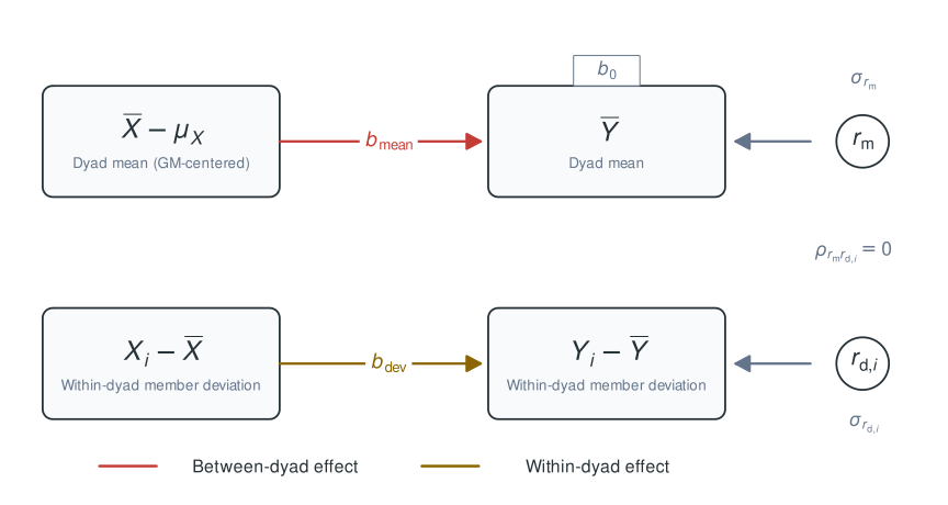
Cross-sectional DIM. The dyad mean has a between-dyad effect, and the within-dyad member deviation has a within-dyad effect. Mean and deviation residuals are uncorrelated under exchangeability. Both members’ residuals and their correlation can be obtained from these residuals.

Uncorrelated $r_{\mathrm{m}}$ and $r_{\mathrm{d},i}$ in the conceptual representation do not imply that the member residuals are independent: the two component variances together determine the covariance between the members’ residuals.

The second diagram translates the same decomposition to the individual-member rows used by the long-format multilevel model. Each member’s outcome is predicted by the dyad mean and that member’s own within-dyad member deviation. Both members share the same two coefficients, so estimation pools information across members under the exchangeability assumptions.

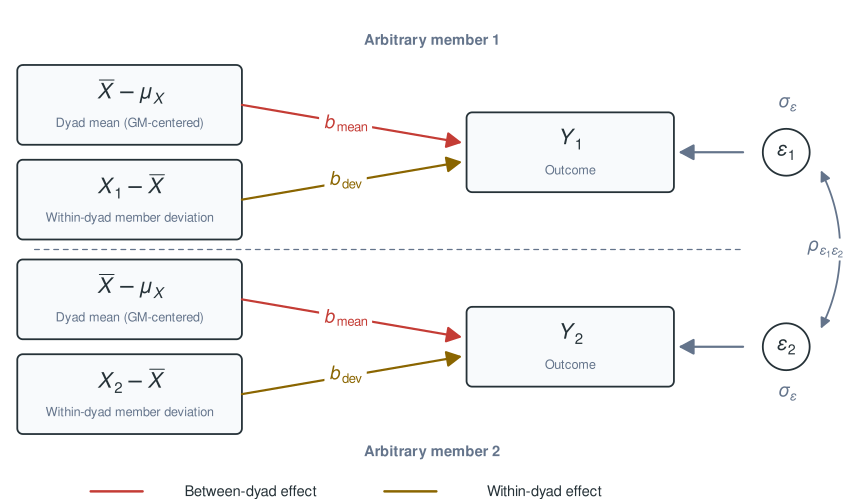
Individual-level representation of the cross-sectional DIM used for the long-format multilevel model.

The resulting estimated fixed effects are a reparameterization of the APIM actor and partner effects (Bolger et al. 2025). And just like the exchangeable APIM, the random-effects structure comprises a dyad-level intercept and a dyad-level difference contrast indexed by .i_diff_assumed_exchangeable_arbitrary. In glmmTMB, with dispformula = ~ 0, these random effects represent the two members’ Gaussian residual variance and covariance.

The intercept and difference contrast are specified as separate random-effects terms. No additional correlation is needed because the two residual variances already determine the partners’ residual correlation. Under exchangeability, the mean-deviation residual correlation is therefore fixed to zero (del Rosario and West 2025).

The full model can be estimated as:

dim_1 <- glmmTMB::glmmTMB(
  satisfaction ~

    # Pooled fixed intercept
    1 +

    # Between-dyad effect
    .i_communication_dyad_mean_gmc +

    # Within-dyad effect
    .i_communication_within_dyad_dev +

    # Residual Gaussian covariance structure
    us(1 | coupleID) +
    us(0 + .i_diff_assumed_exchangeable_arbitrary | coupleID)
  , dispformula = ~ 0
  , family = gaussian()
  , data = cross_exchangeable_data
)

summary(dim_1)
#>  Family: gaussian  ( identity )
#> Formula:          
#> satisfaction ~ 1 + .i_communication_dyad_mean_gmc + .i_communication_within_dyad_dev +  
#>     us(1 | coupleID) + us(0 + .i_diff_assumed_exchangeable_arbitrary |  
#>     coupleID)
#> Dispersion:                    ~0
#> Data: cross_exchangeable_data
#> 
#>       AIC       BIC    logLik -2*log(L)  df.resid 
#>     604.0     619.8    -297.0     594.0       171 
#> 
#> Random effects:
#> 
#> Conditional model:
#>  Groups     Name                                   Variance Std.Dev.
#>  coupleID   (Intercept)                            0.6346   0.7966  
#>  coupleID.1 .i_diff_assumed_exchangeable_arbitrary 1.1532   1.0739  
#> Number of obs: 176, groups:  coupleID, 88
#> 
#> Conditional model:
#>                                  Estimate Std. Error z value Pr(>|z|)    
#> (Intercept)                       5.04066    0.08492   59.36   <2e-16 ***
#> .i_communication_dyad_mean_gmc    1.99563    0.07797   25.59   <2e-16 ***
#> .i_communication_within_dyad_dev  1.51989    0.14406   10.55   <2e-16 ***
#> ---
#> Signif. codes:  0 '***' 0.001 '**' 0.01 '*' 0.05 '.' 0.1 ' ' 1

The same mean-and-deviation diagram can now be labelled with the estimated fixed effects and residual-component standard deviations:

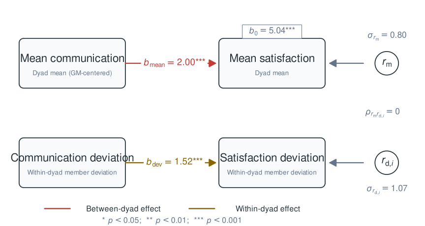
Estimated fixed effects and residual-component standard deviations from the cross-sectional Gaussian DIM in its mean-and-deviation representation. The intercept belongs to the outcome-mean equation.

Under these exchangeability constraints, the Gaussian DIM is algebraically equivalent to the reduced, label-invariant Dyadic Score Model (DSM) (Iida et al. 2018). Compared to a full DSM, the DIM’s exchangeability constraints fix the outcome-deviation intercept and both cross-paths to zero and constrain the mean and deviation residual components to be uncorrelated (see the diagrams here and compare them with the conceptual DSM diagrams).

Model interpretation

Therefore, each coefficient has both an individual-member interpretation and an equivalent dyad mean/difference interpretation.

In this Gaussian model, fixed coefficients are interpreted in units of the outcome, e.g., “satisfaction”:

• The intercept (about 5.04) is the expected satisfaction of either member, and therefore the expected couple-average satisfaction, when both members’ communication equals the sample grand mean.

• The between-dyad effect estimate (about 2.00) means that, comparing couples with the same communication difference between partners, a one-point higher couple-average communication level is associated with a 2.00-point higher expected couple-average satisfaction. Equivalently, each member’s expected satisfaction is 2.00 points higher.

• The within-dyad effect estimate (about 1.52) means that a one-point difference in communication between partners is associated with a 1.52-point difference in their expected satisfaction, holding their average communication constant. In member terms, suppose one member is 0.5 points above the dyad mean and the other is 0.5 points below it. Their expected satisfaction is then 0.76 points above and below the couple’s predicted mean, respectively, so they are expected to differ by 1.52 points in satisfaction.

Because the Gaussian DIM is the exchangeability-constrained version of the full DSM, exchangeability can also be tested by comparing these nested models. This is equivalent to the comparison shown in Testing distinguishability in the APIM vignette.

Demonstrating model equivalence to APIM

The same model can be written in APIM form. Since we have requested both sets of variables from prepare_interdep_data(), we can fit one directly. For more guidance on APIM specifications and different models, see the Actor-Partner Interdependence Model vignette.

apim_1 <- glmmTMB::glmmTMB(
  satisfaction ~ 1 +

    # Fixed effects APIM
    .i_communication_actor + .i_communication_partner +

    # Since both models are equivalent, the same random-effects structure
    # can be used. See the APIM vignette to learn how to back-transform
    # these blocks to a full actor-partner covariance matrix.
    us(1 | coupleID) +
    us(0 + .i_diff_assumed_exchangeable_arbitrary | coupleID)
  , dispformula = ~ 0
  , family = gaussian()
  , data = cross_exchangeable_data
)

The two models have identical fit statistics:

data.frame(
  model = c("DIM", "APIM"),
  AIC = c(AIC(dim_1), AIC(apim_1)),
  BIC = c(BIC(dim_1), BIC(apim_1)),
  logLik = c(as.numeric(logLik(dim_1)), as.numeric(logLik(apim_1)))
)
#>   model      AIC      BIC    logLik
#> 1   DIM 603.9834 619.8358 -296.9917
#> 2  APIM 603.9834 619.8358 -296.9917

This demonstrates that the same statistical model is being estimated with different parameterizations and coefficient interpretations.

Once APIM estimates are present, one can easily obtain DIM estimates, and the other way around. Let $b_{\mathrm{actor}}$ and $b_{\mathrm{partner}}$ denote the APIM actor and partner slopes, and let $b_{\mathrm{mean}}$ and $b_{\mathrm{dev}}$ denote the DIM between-dyad and within-dyad slopes. They relate as follows:

$$b_{\mathrm{mean}} = b_{\mathrm{actor}} + b_{\mathrm{partner}}$$

and

$$b_{\mathrm{dev}} = b_{\mathrm{actor}} - b_{\mathrm{partner}}$$

Conversely:

$$b_{\mathrm{actor}} = \frac{b_{\mathrm{mean}} + b_{\mathrm{dev}}}{2}$$

and

$$b_{\mathrm{partner}} = \frac{b_{\mathrm{mean}} - b_{\mathrm{dev}}}{2}$$

In this example we can see that the transformations work:

apim_coef <- glmmTMB::fixef(apim_1)$cond
dim_coef <- glmmTMB::fixef(dim_1)$cond

b_actor <- apim_coef[[".i_communication_actor"]]
b_partner <- apim_coef[[".i_communication_partner"]]

b_mean <- dim_coef[[".i_communication_dyad_mean_gmc"]]
b_dev <- dim_coef[[".i_communication_within_dyad_dev"]]


cat("From APIM model:\n",
     "  actor effect:                  ", round(b_actor, 3), "\n",
     "  partner effect:                ", round(b_partner, 3), "\n\n",

     "DIM transformation:\n",
     "  b_mean = b_actor + b_partner:  ", round(b_actor + b_partner, 3), "\n",
     "  b_dev = b_actor - b_partner:   ", round(b_actor - b_partner, 3), "\n\n",

     "From DIM model:\n",
     "  between-dyad effect:           ", round(b_mean, 3), "\n",
     "  within-dyad effect:            ", round(b_dev, 3), "\n"
)
#> From APIM model:
#>    actor effect:                   1.758 
#>    partner effect:                 0.238 
#> 
#>  DIM transformation:
#>    b_mean = b_actor + b_partner:   1.996 
#>    b_dev = b_actor - b_partner:    1.52 
#> 
#>  From DIM model:
#>    between-dyad effect:            1.996 
#>    within-dyad effect:             1.52

The DIM and APIM intercepts are not expected to be equal because the DIM dyad mean is grand-mean centered, whereas the APIM predictors retain their original scale.

Why Are These Models Equivalent? Exploring the Reparameterization

An intuitive way to think about this is:

• When the dyad mean goes up by 1 unit while the difference between partners remains stable, both partners’ values must go up by 1. Both the actor and partner effects therefore contribute, which is why the between-dyad effect is the actor effect + the partner effect.

• When a person’s deviation from the dyad mean goes up by 1 unit while the dyad mean remains constant, the other partner’s value must go down by 1 unit. The actor value therefore changes by +1 and the partner value by -1, which is why the within-dyad effect is the actor effect - the partner effect.

The grid below shows the same predictor values in both coordinate systems. The horizontal and vertical axes are actor and partner values centered at the sample grand mean. The diagonal axes are their dyad mean and within-dyad member deviation.

The displayed actor and partner slopes are read from the fitted APIM. The DIM slopes are their exact sum-and-difference transformation; the directly fitted DIM estimates above confirm the equivalence. Both forms therefore make the same change in the linear predictor relative to the grand-mean reference. The intercept is omitted from both displayed equations.

Communication coordinates Reset

APIM coordinates

Grand-mean-centered actor, x_actor

0.00

Grand-mean-centered partner, x_partner

0.00

DIM coordinates

Dyad mean, x_mean

0.00

Within-dyad member deviation, x_dev

0.00

x_mean = (x_actor + x_partner) / 2 x_dev = (x_actor − x_partner) / 2

APIM

DIM

Shared dyad levelBoth members +1

b_mean = a + p

Within-dyad member deviationActor +1, partner −1

b_dev = a − p

Drag the dot or move either set of sliders. Both equations give the same fitted change in the linear predictor.

Random-effect transformation

The DIM and APIM models above already use the same sum-and-difference random-effects parameterization (del Rosario and West 2025). See the exchangeable residual-structure section of the APIM vignette for the derivation and back-transformation to the member-level covariance matrix.

Intensive Longitudinal DIM

For longitudinal DIM, predictors are decomposed into within-person and between-person components before the dyadic decomposition (Bolger and Laurenceau 2013; Gistelinck and Loeys 2020). The default "auto" selects "time_2l" when both time and predictors are supplied. It also retains raw dyad-occasion means and within-dyad member deviations. The decomposed columns used below are:

1. The cwp dyad mean captures a shared occasion-specific shift from the two members’ usual levels (shared occasion-level variation).
2. The cwp within-dyad member deviation captures which member is further above or below their own usual level on that occasion.
3. The cbp dyad mean captures the dyad’s shared usual level relative to the sample’s grand mean (stable between-dyad differences).
4. The cbp within-dyad member deviation captures each member’s stable difference from the dyad’s usual level.

The cbp terms use each member’s mean across the observed occasions to estimate that member’s longer-run usual level. With few occasions (small $T$), especially when the predictor has low stability over time, these person means can be unreliable. The associated between-person estimates can therefore be biased or imprecise, so they should be interpreted cautiously (Gottfredson 2019).

Use temporal_predictor_decomposition = "none" to construct only the raw dyad-occasion mean and within-dyad member deviation.

ild_exchangeable_data <- prepare_interdep_data(
  example_dyadic_ILD,
  group = coupleID,
  member = personID,
  time = diaryday,
  predictors = provided_support,
  model_type = c("apim", "dim"),
  seed = 123
)

print(ild_exchangeable_data)
#> # interdep data
#> # Rows: 1120 | Dyads: 40 | Intensive longitudinal: yes
#> # Structure: group = coupleID, member = personID, time = diaryday
#> #
#> # Dyad compositions:
#> # assumed_exchangeable exchangeable 40 dyads
#> #
#> # Added columns:
#> #   .i_composition                 inferred dyad composition
#> #   .i_composition_role            composition-specific member role
#> #   .i_is_{comp-role}              composition-role indicator columns
#> #   .i_diff_{comp}                 composition-specific sum-diff contrasts with
#> #                                  arbitrary direction; 0 for distinguishable
#> #                                  dyads or other exchangeable compositions
#> #   .i_{pred}_cwp                  within-person predictor: momentary
#> #                                  deviations from each person's usual level
#> #   .i_{pred}_cbp                  between-person predictor: stable differences
#> #                                  from the average person's usual level
#> #   .i_{pred}_actor                APIM actor predictor: actor's original
#> #                                  predictor values
#> #   .i_{pred}_partner              APIM partner predictor: partner's original
#> #                                  predictor values
#> #   .i_{pred}_cwp_actor            APIM within-person actor predictor: actor's
#> #                                  momentary deviations from their usual level
#> #   .i_{pred}_cwp_partner          APIM within-person partner predictor:
#> #                                  partner's momentary deviations from their
#> #                                  usual level
#> #   .i_{pred}_cbp_actor            APIM between-person actor predictor: actor's
#> #                                  stable difference from the average person's
#> #                                  usual level
#> #   .i_{pred}_cbp_partner          APIM between-person partner predictor:
#> #                                  partner's stable difference from the average
#> #                                  person's usual level
#> #   .i_{pred}_dyad_mean_gmc        dyad-mean predictor: dyad's average
#> #                                  predictor level, grand-mean centered
#> #   .i_{pred}_within_dyad_dev      DIM within-dyad member-deviation predictor:
#> #                                  member's difference from the dyad mean
#> #   .i_{pred}_cwp_dyad_mean        within-person dyad-mean predictor: shared
#> #                                  momentary deviations in the dyad
#> #   .i_{pred}_cwp_within_dyad_dev  DIM within-person, within-dyad
#> #                                  member-deviation predictor: member's
#> #                                  momentary deviation from the dyad mean
#> #   .i_{pred}_cbp_dyad_mean        between-person dyad-mean predictor: dyad's
#> #                                  stable usual level, grand-mean centered
#> #   .i_{pred}_cbp_within_dyad_dev  DIM between-person, within-dyad
#> #                                  member-deviation predictor: member's stable
#> #                                  difference from the dyad's usual level
#> #
#> # A tibble: 1,120 × 24
#>    personID coupleID diaryday gender closeness provided_support .i_composition  
#>       <int>    <int>    <int> <fct>      <dbl>            <dbl> <fct>           
#>  1        1        1        0 female      5.03             4.30 assumed_exchang…
#>  2        1        1        1 female      5.64             4.24 assumed_exchang…
#>  3        1        1        2 female      5.49             3.54 assumed_exchang…
#>  4        1        1        3 female      6.71             5.04 assumed_exchang…
#>  5        1        1        4 female      5.61             4.74 assumed_exchang…
#>  6        1        1        5 female      6.11             4.72 assumed_exchang…
#>  7        1        1        6 female      6.96             5.12 assumed_exchang…
#>  8        1        1        7 female      7.03             5.21 assumed_exchang…
#>  9        1        1        8 female      8.07             5.20 assumed_exchang…
#> 10        1        1        9 female      4.87             4.69 assumed_exchang…
#> # ℹ 1,110 more rows
#> # ℹ 17 more variables: .i_composition_role <fct>,
#> #   .i_is_assumed_exchangeable <dbl>,
#> #   .i_diff_assumed_exchangeable_arbitrary <dbl>,
#> #   .i_provided_support_cwp <dbl>, .i_provided_support_cbp <dbl>,
#> #   .i_provided_support_actor <dbl>, .i_provided_support_partner <dbl>,
#> #   .i_provided_support_cwp_actor <dbl>, …

The example below estimates same-day associations between support and closeness and includes diaryday to adjust for a linear trend across the study.

dim_ILD <- glmmTMB::glmmTMB(
  closeness ~
    1 +

    diaryday +

    # Within-person DIM
    .i_provided_support_cwp_dyad_mean +
    .i_provided_support_cwp_within_dyad_dev +

    # Between-person DIM
    .i_provided_support_cbp_dyad_mean +
    .i_provided_support_cbp_within_dyad_dev +

    # Stable exchangeable dyad-level covariance
    us(1 | coupleID) +
    us(0 + .i_diff_assumed_exchangeable_arbitrary | coupleID) +

    # Residual (same-day) exchangeable dyad-level covariance
    us(1 | coupleID:diaryday) +
    us(0 + .i_diff_assumed_exchangeable_arbitrary | coupleID:diaryday)

  , dispformula = ~ 0
  , family = gaussian()
  , data = ild_exchangeable_data
)

summary(dim_ILD)
#>  Family: gaussian  ( identity )
#> Formula:          
#> closeness ~ 1 + diaryday + .i_provided_support_cwp_dyad_mean +  
#>     .i_provided_support_cwp_within_dyad_dev + .i_provided_support_cbp_dyad_mean +  
#>     .i_provided_support_cbp_within_dyad_dev + us(1 | coupleID) +  
#>     us(0 + .i_diff_assumed_exchangeable_arbitrary | coupleID) +  
#>     us(1 | coupleID:diaryday) + us(0 + .i_diff_assumed_exchangeable_arbitrary |  
#>     coupleID:diaryday)
#> Dispersion:                 ~0
#> Data: ild_exchangeable_data
#> 
#>       AIC       BIC    logLik -2*log(L)  df.resid 
#>    2977.2    3026.6   -1478.6    2957.2      1024 
#> 
#> Random effects:
#> 
#> Conditional model:
#>  Groups              Name                                   Variance Std.Dev.
#>  coupleID            (Intercept)                            0.5254   0.7248  
#>  coupleID.1          .i_diff_assumed_exchangeable_arbitrary 0.6416   0.8010  
#>  coupleID.diaryday   (Intercept)                            0.3185   0.5643  
#>  coupleID.diaryday.1 .i_diff_assumed_exchangeable_arbitrary 0.5184   0.7200  
#> Number of obs: 1034, groups:  coupleID, 40; coupleID:diaryday, 517
#> 
#> Conditional model:
#>                                          Estimate Std. Error z value Pr(>|z|)
#> (Intercept)                              5.079988   0.124223   40.89  < 2e-16
#> diaryday                                -0.008077   0.006234   -1.30   0.1951
#> .i_provided_support_cwp_dyad_mean        0.487152   0.041725   11.68  < 2e-16
#> .i_provided_support_cwp_within_dyad_dev  0.055002   0.072173    0.76   0.4460
#> .i_provided_support_cbp_dyad_mean        1.510701   0.193894    7.79 6.63e-15
#> .i_provided_support_cbp_within_dyad_dev  0.776673   0.302810    2.56   0.0103
#>                                            
#> (Intercept)                             ***
#> diaryday                                   
#> .i_provided_support_cwp_dyad_mean       ***
#> .i_provided_support_cwp_within_dyad_dev    
#> .i_provided_support_cbp_dyad_mean       ***
#> .i_provided_support_cbp_within_dyad_dev *  
#> ---
#> Signif. codes:  0 '***' 0.001 '**' 0.01 '*' 0.05 '.' 0.1 ' ' 1

Interpretation of concurrent ILD DIM coefficients

The same mean-and-deviation interpretation applies longitudinally. Coefficients of dyad means describe both expected individual outcomes and expected couple-average outcomes. Coefficients of within-dyad member deviations describe both members’ deviations and their expected difference.

• The cbp dyad-mean estimate (about 1.51) means that, comparing couples whose average usual support differs by one point while holding the stable difference between partners constant, expected couple-average closeness is 1.51 points higher for the higher-support couple. Equivalently, each member is expected to report 1.51 points higher closeness.

• The cwp dyad-mean estimate (about 0.49) means that when both members are one point above their respective usual support levels, each member’s expected closeness is 0.49 points higher than when both are at their usual levels, holding the difference between their momentary deviations constant. Equivalently, expected couple-average closeness is 0.49 points higher on that occasion.

• The cbp within-dyad member-deviation estimate (about 0.78) means that if partners differ by one point in their usual support levels, they are expected to differ by 0.78 points in closeness, holding the couple’s average usual support and the other predictors constant. In member terms, suppose one member is 0.5 points above the couple’s average usual support and the other is 0.5 points below it. Their expected closeness is then 0.39 points above and below the couple’s predicted mean, respectively.

• The cwp within-dyad member-deviation estimate (about 0.06) means that if one partner’s momentary deviation from usual support is one point higher than the other partner’s deviation, they are expected to differ by 0.06 points in closeness, holding the occasion-specific dyad mean and the other predictors constant. In member terms, suppose their momentary deviations are 0.5 points above and below the occasion-specific dyad mean. Their expected closeness is then 0.03 points above and below the couple’s predicted mean, respectively.

Equivalence of APIM and DIM in ILD

The equivalent APIM uses actor and partner effects on both levels:

apim_ILD <- glmmTMB::glmmTMB(
  closeness ~
    1 +

    diaryday +

    # Within-person APIM
    .i_provided_support_cwp_actor +
    .i_provided_support_cwp_partner +

    # Between-person APIM
    .i_provided_support_cbp_actor +
    .i_provided_support_cbp_partner +

    # Stable exchangeable dyad-level covariance
    us(1 | coupleID)  + us(0 + .i_diff_assumed_exchangeable_arbitrary | coupleID) +

    # Residual (same-day) exchangeable dyad-level covariance
    us(1 | coupleID:diaryday) +
    us(0 + .i_diff_assumed_exchangeable_arbitrary | coupleID:diaryday)

  , dispformula = ~ 0
  , family = gaussian()
  , data = ild_exchangeable_data
)

The two ILD models again have identical fit statistics:

data.frame(
  model = c("DIM", "APIM"),
  AIC = c(AIC(dim_ILD), AIC(apim_ILD)),
  BIC = c(BIC(dim_ILD), BIC(apim_ILD)),
  logLik = c(as.numeric(logLik(dim_ILD)), as.numeric(logLik(apim_ILD)))
)
#>   model      AIC      BIC    logLik
#> 1   DIM 2977.225 3026.637 -1478.613
#> 2  APIM 2977.225 3026.637 -1478.613

The equivalence holds separately for the within-person (cwp) and between-person (cbp) predictor components. For the within-person component:

$$b_{\mathrm{cwp,mean}} = b_{\mathrm{cwp,actor}} + b_{\mathrm{cwp,partner}}$$

$$b_{\mathrm{cwp,diff}} = b_{\mathrm{cwp,actor}} - b_{\mathrm{cwp,partner}}$$

For the between-person component:

$$b_{\mathrm{cbp,mean}} = b_{\mathrm{cbp,actor}} + b_{\mathrm{cbp,partner}}$$

$$b_{\mathrm{cbp,diff}} = b_{\mathrm{cbp,actor}} - b_{\mathrm{cbp,partner}}$$

This also means that an APIM parameterization can be used on one level and a DIM parameterization on the other. For example:

apim_dim_ILD <- glmmTMB::glmmTMB(
  closeness ~
    1 +

    diaryday +

    # Within-person APIM
    .i_provided_support_cwp_actor +
    .i_provided_support_cwp_partner +

    # Between-person DIM
    .i_provided_support_cbp_dyad_mean +
    .i_provided_support_cbp_within_dyad_dev +

    # Stable exchangeable dyad-level covariance
    us(1 | coupleID)  + us(0 + .i_diff_assumed_exchangeable_arbitrary | coupleID) +

    # Same-day exchangeable dyad-level covariance
    us(1 | coupleID:diaryday) +
    us(0 + .i_diff_assumed_exchangeable_arbitrary | coupleID:diaryday)

  , dispformula = ~ 0
  , family = gaussian()
  , data = ild_exchangeable_data
)

This mixed parameterization still estimates the same model:

data.frame(
  model = c("DIM within / DIM between", "APIM within / APIM between", "APIM within / DIM between"),
  AIC = c(AIC(dim_ILD), AIC(apim_ILD), AIC(apim_dim_ILD)),
  BIC = c(BIC(dim_ILD), BIC(apim_ILD), BIC(apim_dim_ILD)),
  logLik = c(
    as.numeric(logLik(dim_ILD)),
    as.numeric(logLik(apim_ILD)),
    as.numeric(logLik(apim_dim_ILD))
  )
)
#>                        model      AIC      BIC    logLik
#> 1   DIM within / DIM between 2977.225 3026.637 -1478.613
#> 2 APIM within / APIM between 2977.225 3026.637 -1478.613
#> 3  APIM within / DIM between 2977.225 3026.637 -1478.613

Including Random Slopes

Random slopes can be included in the DIM by adding the corresponding within-person effects to the stable dyad-level random-effect blocks:

The following syntax illustrates the full random-slope specification. It is not fitted here because the example data do not support this complex random-effects structure.

dim_ILD_random <- glmmTMB::glmmTMB(
  closeness ~
    1 +

    diaryday +

    # Within-person DIM
    .i_provided_support_cwp_dyad_mean +
    .i_provided_support_cwp_within_dyad_dev +

    # Between-person DIM
    .i_provided_support_cbp_dyad_mean +
    .i_provided_support_cbp_within_dyad_dev +

    # Stable dyad-level covariance with within-person random slopes
    us(1 +
       .i_provided_support_cwp_dyad_mean +
       .i_provided_support_cwp_within_dyad_dev
     | coupleID)  +
    us(0 +
       .i_diff_assumed_exchangeable_arbitrary +
       .i_diff_assumed_exchangeable_arbitrary:.i_provided_support_cwp_dyad_mean +
       .i_diff_assumed_exchangeable_arbitrary:.i_provided_support_cwp_within_dyad_dev
     | coupleID) +

    # Same-day exchangeable dyad-level covariance
    us(1 | coupleID:diaryday) +
    us(0 + .i_diff_assumed_exchangeable_arbitrary | coupleID:diaryday)

  , dispformula = ~ 0
  , family = gaussian()
  , data = ild_exchangeable_data
)

The first stable dyad-level random effects block contains the shared DIM intercept, dyad-mean slope, and within-dyad member-deviation slope. The second block contains their member-difference counterparts, included through the .i_diff_* interactions. These uncorrelated blocks allow the two members to have different random slopes while preserving exchangeability.

Transforming DIM random slopes to APIM slopes

Applying the same transformation to the random-slope coefficients proceeds in two steps. First, transform the DIM dyad-mean and within-dyad member-deviation random slopes into APIM actor and partner random slopes. Random effects use $u$, with subscripts that write out actor, partner, mean, and dev. For the shared block,

$$u_{\mathrm{actor},j} = \frac{u_{\mathrm{mean},j} + u_{\mathrm{dev},j}}{2}, \qquad u_{\mathrm{partner},j} = \frac{u_{\mathrm{mean},j} - u_{\mathrm{dev},j}}{2},$$

and for the .i_diff_* block, marked by a tilde,

$$\widetilde{u}_{\mathrm{actor},j} = \frac{\widetilde{u}_{\mathrm{mean},j} + \widetilde{u}_{\mathrm{dev},j}}{2}, \qquad \widetilde{u}_{\mathrm{partner},j} = \frac{\widetilde{u}_{\mathrm{mean},j} - \widetilde{u}_{\mathrm{dev},j}}{2}.$$

The shared and .i_diff_* random intercepts remain unchanged.

We now have the shared and .i_diff_* actor and partner effects which are then back-transformed into the complete and more readily interpretable member-specific actor-partner covariance matrix. This is described in the exchangeable random-slope back-transformation in the APIM vignette.

Dynamic ILD DIM example

The ILD models above do not model residual serial dependence. One way to model dynamics or to account for temporal dependency is to include lagged outcomes as predictors.

Note: Dynamic models, especially with small time series, are subject to bias. This, and the choice between raw and within-person-centered outcome lags, are addressed in the APIM vignette’s discussion of dynamic models.

Brief example to obtain lagged raw and within-person centered versions of the outcome:

ild_exchangeable_data_dynamic <- prepare_interdep_data(
  example_dyadic_ILD,
  group = coupleID,
  member = personID,
  time = diaryday,
  predictors = c(provided_support, closeness),
  lag_predictors = closeness,
  model_type = "dim",
  seed = 123
)

print(ild_exchangeable_data_dynamic)
#> # interdep data
#> # Rows: 1120 | Dyads: 40 | Intensive longitudinal: yes
#> # Structure: group = coupleID, member = personID, time = diaryday
#> #
#> # Dyad compositions:
#> # assumed_exchangeable exchangeable 40 dyads
#> #
#> # Added columns:
#> #   .i_composition                      inferred dyad composition
#> #   .i_composition_role                 composition-specific member role
#> #   .i_is_{comp-role}                   composition-role indicator columns
#> #   .i_diff_{comp}                      composition-specific sum-diff contrasts
#> #                                       with arbitrary direction; 0 for
#> #                                       distinguishable dyads or other
#> #                                       exchangeable compositions
#> #   .i_{pred}_lag1                      lag-1 raw predictor values
#> #   .i_{pred}_cwp                       within-person predictor: momentary
#> #                                       deviations from each person's usual
#> #                                       level
#> #   .i_{pred}_cwp_lag1                  lag-1 within-person predictor:
#> #                                       momentary deviations from each person's
#> #                                       usual level
#> #   .i_{pred}_cbp                       between-person predictor: stable
#> #                                       differences from the average person's
#> #                                       usual level
#> #   .i_{pred}_dyad_mean_gmc             dyad-mean predictor: dyad's average
#> #                                       predictor level, grand-mean centered
#> #   .i_{pred}_dyad_mean_gmc_lag1        lag-1 dyad-mean predictor: dyad's
#> #                                       average predictor level, grand-mean
#> #                                       centered
#> #   .i_{pred}_within_dyad_dev           DIM within-dyad member-deviation
#> #                                       predictor: member's difference from the
#> #                                       dyad mean
#> #   .i_{pred}_within_dyad_dev_lag1      lag-1 DIM within-dyad member-deviation
#> #                                       predictor: member's difference from the
#> #                                       dyad mean
#> #   .i_{pred}_cwp_dyad_mean             within-person dyad-mean predictor:
#> #                                       shared momentary deviations in the dyad
#> #   .i_{pred}_cwp_dyad_mean_lag1        lag-1 within-person dyad-mean
#> #                                       predictor: shared momentary deviations
#> #                                       in the dyad
#> #   .i_{pred}_cwp_within_dyad_dev       DIM within-person, within-dyad
#> #                                       member-deviation predictor: member's
#> #                                       momentary deviation from the dyad mean
#> #   .i_{pred}_cwp_within_dyad_dev_lag1  lag-1 DIM within-person, within-dyad
#> #                                       member-deviation predictor: member's
#> #                                       momentary deviation from the dyad mean
#> #   .i_{pred}_cbp_dyad_mean             between-person dyad-mean predictor:
#> #                                       dyad's stable usual level, grand-mean
#> #                                       centered
#> #   .i_{pred}_cbp_within_dyad_dev       DIM between-person, within-dyad
#> #                                       member-deviation predictor: member's
#> #                                       stable difference from the dyad's usual
#> #                                       level
#> #
#> # A tibble: 1,120 × 32
#>    personID coupleID diaryday gender closeness provided_support .i_composition  
#>       <int>    <int>    <int> <fct>      <dbl>            <dbl> <fct>           
#>  1        1        1        0 female      5.03             4.30 assumed_exchang…
#>  2        1        1        1 female      5.64             4.24 assumed_exchang…
#>  3        1        1        2 female      5.49             3.54 assumed_exchang…
#>  4        1        1        3 female      6.71             5.04 assumed_exchang…
#>  5        1        1        4 female      5.61             4.74 assumed_exchang…
#>  6        1        1        5 female      6.11             4.72 assumed_exchang…
#>  7        1        1        6 female      6.96             5.12 assumed_exchang…
#>  8        1        1        7 female      7.03             5.21 assumed_exchang…
#>  9        1        1        8 female      8.07             5.20 assumed_exchang…
#> 10        1        1        9 female      4.87             4.69 assumed_exchang…
#> # ℹ 1,110 more rows
#> # ℹ 25 more variables: .i_composition_role <fct>,
#> #   .i_is_assumed_exchangeable <dbl>,
#> #   .i_diff_assumed_exchangeable_arbitrary <dbl>,
#> #   .i_provided_support_cwp <dbl>, .i_provided_support_cbp <dbl>,
#> #   .i_closeness_cwp <dbl>, .i_closeness_cbp <dbl>, .i_closeness_lag1 <dbl>,
#> #   .i_closeness_cwp_lag1 <dbl>, .i_provided_support_dyad_mean_gmc <dbl>, …

Lags are matched at exactly diaryday - 1, so omitted diary days are not bridged.

The raw lagged outcome scores can be included in the model as follows:

dim_ILD_lag_raw <- glmmTMB::glmmTMB(
  closeness ~
    1 +

    # Raw lagged outcomes
    .i_closeness_dyad_mean_gmc_lag1 + .i_closeness_within_dyad_dev_lag1 +

    diaryday +

    # Within-person DIM
    .i_provided_support_cwp_dyad_mean +
    .i_provided_support_cwp_within_dyad_dev +

    # Between-person DIM
    .i_provided_support_cbp_dyad_mean +
    .i_provided_support_cbp_within_dyad_dev +

    # Stable exchangeable dyad-level covariance
    us(1 | coupleID)  +
    us(0 + .i_diff_assumed_exchangeable_arbitrary | coupleID) +

    # Same-day exchangeable dyad-level covariance
    us(1 | coupleID:diaryday) +
    us(0 + .i_diff_assumed_exchangeable_arbitrary | coupleID:diaryday)

  , dispformula = ~ 0
  , family = gaussian()
  , data = ild_exchangeable_data_dynamic

  # The model did not converge with the default optimizer
  , control = glmmTMB::glmmTMBControl(
      optimizer = stats::optim,
      optArgs = list(method = "BFGS")
    )
)

summary(dim_ILD_lag_raw)
#>  Family: gaussian  ( identity )
#> Formula:          
#> closeness ~ 1 + .i_closeness_dyad_mean_gmc_lag1 + .i_closeness_within_dyad_dev_lag1 +  
#>     diaryday + .i_provided_support_cwp_dyad_mean + .i_provided_support_cwp_within_dyad_dev +  
#>     .i_provided_support_cbp_dyad_mean + .i_provided_support_cbp_within_dyad_dev +  
#>     us(1 | coupleID) + us(0 + .i_diff_assumed_exchangeable_arbitrary |  
#>     coupleID) + us(1 | coupleID:diaryday) + us(0 + .i_diff_assumed_exchangeable_arbitrary |  
#>     coupleID:diaryday)
#> Dispersion:                 ~0
#> Data: ild_exchangeable_data_dynamic
#> 
#>       AIC       BIC    logLik -2*log(L)  df.resid 
#>    2646.3    2704.2   -1311.1    2622.3       914 
#> 
#> Random effects:
#> 
#> Conditional model:
#>  Groups              Name                                   Variance Std.Dev.
#>  coupleID            (Intercept)                            0.4165   0.6453  
#>  coupleID.1          .i_diff_assumed_exchangeable_arbitrary 0.5061   0.7114  
#>  coupleID.diaryday   (Intercept)                            0.2984   0.5462  
#>  coupleID.diaryday.1 .i_diff_assumed_exchangeable_arbitrary 0.5222   0.7227  
#> Number of obs: 926, groups:  coupleID, 40; coupleID:diaryday, 463
#> 
#> Conditional model:
#>                                          Estimate Std. Error z value Pr(>|z|)
#> (Intercept)                              5.103583   0.115953   44.01  < 2e-16
#> .i_closeness_dyad_mean_gmc_lag1          0.084935   0.044485    1.91   0.0562
#> .i_closeness_within_dyad_dev_lag1        0.107830   0.051833    2.08   0.0375
#> diaryday                                -0.010202   0.006877   -1.48   0.1380
#> .i_provided_support_cwp_dyad_mean        0.459125   0.042955   10.69  < 2e-16
#> .i_provided_support_cwp_within_dyad_dev  0.052021   0.076426    0.68   0.4961
#> .i_provided_support_cbp_dyad_mean        1.390956   0.186473    7.46  8.7e-14
#> .i_provided_support_cbp_within_dyad_dev  0.704069   0.275077    2.56   0.0105
#>                                            
#> (Intercept)                             ***
#> .i_closeness_dyad_mean_gmc_lag1         .  
#> .i_closeness_within_dyad_dev_lag1       *  
#> diaryday                                   
#> .i_provided_support_cwp_dyad_mean       ***
#> .i_provided_support_cwp_within_dyad_dev    
#> .i_provided_support_cbp_dyad_mean       ***
#> .i_provided_support_cbp_within_dyad_dev *  
#> ---
#> Signif. codes:  0 '***' 0.001 '**' 0.01 '*' 0.05 '.' 0.1 ' ' 1

The lagged dyad-mean coefficient describes how a one-point higher shared prior outcome level relates to both members’ current outcomes. The lagged within-dyad member-deviation coefficient describes how a one-point prior difference between partners relates to their current expected difference.

All predictor effects in this model are conditional on both members’ prior outcomes.

---

Return to the Actor-Partner Interdependence Model vignette, see the Mixed-Composition APIM vignette or the Dyadic Score Model vignette for related model specifications, or return to the Overview.

References

Bolger, Niall, and Jean-Philippe Laurenceau. 2013. Intensive Longitudinal Methods: An Introduction to Diary and Experience Sampling Research. Guilford Press. https://www.guilford.com/books/Intensive-Longitudinal-Methods/Bolger-Laurenceau/9781462506781.

Bolger, Niall, Jean-Philippe Laurenceau, and Ana DiGiovanni. 2025. “Unified Analysis Model for Indistinguishable and Distinguishable Dyads.” Innovations in Interpersonal Relationships and Health Research: Advancing the Integration of Interdisciplinary Approaches to Dyadic Behavior Change. https://doi.org/10.17605/OSF.IO/WYDCJ.

Gistelinck, Fien, and Tom Loeys. 2020. “Multilevel Autoregressive Models for Longitudinal Dyadic Data.” TPM - Testing, Psychometrics, Methodology in Applied Psychology 27 (3): 433–52. https://doi.org/10.4473/TPM27.3.7.

Gottfredson, Nisha C. 2019. “A Straightforward Approach for Coping with Unreliability of Person Means When Parsing Within-Person and Between-Person Effects in Longitudinal Studies.” Addictive Behaviors 94: 156–61. https://doi.org/10.1016/j.addbeh.2018.09.031.

Iida, Masumi, Gwendolyn Seidman, and Patrick E. Shrout. 2018. “Models of Interdependent Individuals Versus Dyadic Processes in Relationship Research.” Journal of Social and Personal Relationships 35 (1): 59–88. https://doi.org/10.1177/0265407517725407.

Kenny, David A, Deborah A Kashy, and William L Cook. 2006. Dyadic Data Analysis. Guilford Press.

Rosario, Kareena S. del, and Tessa V. West. 2025. “A Practical Guide to Specifying Random Effects in Longitudinal Dyadic Multilevel Modeling.” Advances in Methods and Practices in Psychological Science 8 (3): 25152459251351286. https://doi.org/10.1177/25152459251351286.