Within- and between-cluster correlations

Repeated observations contain at least two kinds of association. A between-cluster correlation asks whether clusters with higher values on one variable also tend to have higher values on another. A within-cluster correlation asks whether deviations from a cluster’s usual level move together. These correlations can differ in size or even have opposite signs, so a single correlation calculated from all rows can be misleading.

This vignette demonstrates the basic wbCorr workflow with repeated measurements nested in people.

A contrasting example

The data below are constructed so that people with higher average x also have higher average y. Within a person, however, occasions with higher x than usual tend to have lower y than usual.

set.seed(2026)

n_people <- 60
n_occasions <- 10
person <- rep(seq_len(n_people), each = n_occasions)

person_x <- rnorm(n_people, sd = 2)
person_y <- 0.8 * person_x + rnorm(n_people, sd = 0.5)
occasion_x <- rnorm(n_people * n_occasions)
occasion_y <- -0.7 * occasion_x + rnorm(n_people * n_occasions, sd = 0.6)

dat <- data.frame(
  person = person,
  x = rep(person_x, each = n_occasions) + occasion_x,
  y = rep(person_y, each = n_occasions) + occasion_y
)

round(cor(dat$x, dat$y), 2)
#> [1] 0.55

The pooled correlation is positive, but it combines the two levels of association.

Separate the two levels

Pass the data and the name of the cluster variable to wbCorr(). Using inference = "none" is convenient when only the coefficients are needed.

library(wbCorr)
#> 
#> wbCorr Loaded

fit <- wbCorr(
  data = dat,
  cluster = "person",
  inference = "none"
)

Inspect the correlation matrices

For interactive use, summary() provides short selectors for the most useful correlation matrices. Request the within-cluster matrix with "w" and the between-cluster matrix with "b".

summary(fit, "w")
#> $within
#>       x     y
#> x  1.00 -0.74
#> y -0.74  1.00
summary(fit, "b")
#> $between
#>      x    y
#> x 1.00 0.88
#> y 0.88 1.00

Here the within-person correlation is negative while the between-person correlation is positive. The distinction answers two different questions; one coefficient should not be substituted for the other.

For a compact combined display, use "wb". Within-cluster correlations appear above the diagonal, between-cluster correlations appear below it, and ICCs appear on the diagonal. Use "bw" to reverse the two triangles.

summary(fit, "wb")
#> $merged_wb
#>        x      y
#> x [0.79]  -0.74
#> y   0.88 [0.77]

Calling print(fit) prints a compact preview of the detailed result tables.

Plot the two levels

The corresponding centered data can be inspected visually.

plot(fit, "within")
#> This may take a while...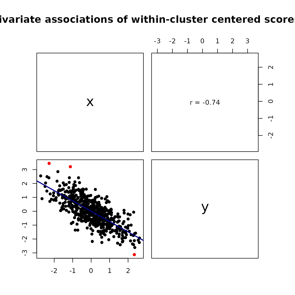

Within-person association after subtracting each person’s variable means.

plot(fit, "between")
#> This may take a while...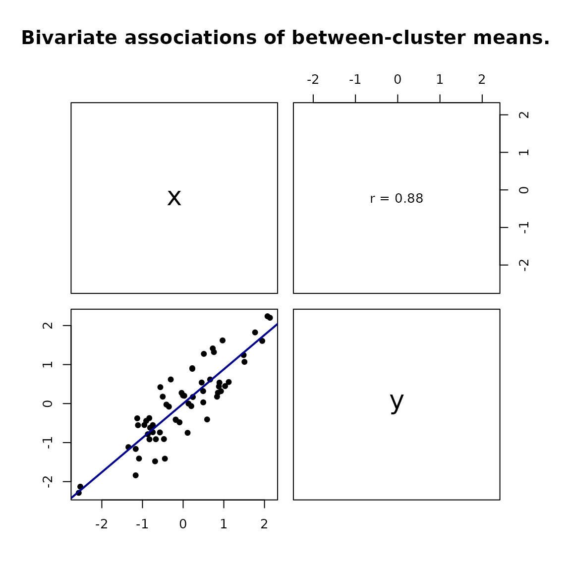

Between-person association among person-level variable means.

Extract results for further work

The summary() shortcuts are convenient for inspection. For programmatic use, get_table() returns the full results and pair-specific diagnostics, while get_matrix() returns selected matrices. Set numeric = TRUE when unrounded numeric coefficients are needed for downstream calculations.

tables <- get_table(fit)
within_table <- tables$within

within_matrix <- get_matrix(fit, "w", numeric = TRUE)$within
merged_matrix <- get_matrix(fit, "wb", numeric = TRUE)$merged_wb

Add uncertainty when needed

By default, Pearson correlations include analytic tests and confidence intervals. These are working approximations for clustered observations. For intervals that preserve top-level dependence, resample whole clusters instead.

set.seed(2026)

fit_boot <- wbCorr(
  data = dat,
  cluster = "person",
  inference = "cluster_bootstrap",
  nboot = 1000
)

Use substantially more than the technical minimum number of bootstrap replicates for substantive analyses, and inspect n_boot_valid in the detailed tables. See ?wbCorr for weighting, centering, missing-data, Spearman, and diagnostic options.